Section11.7Directional Derivatives and the Gradient
Motivating Questions
The partial derivatives of a function \(f\) tell us the rate of change of \(f\) in the direction of the coordinate axes. How can we measure the rate of change of \(f\) in other directions?
The partial derivatives of a multivariable function tell us the instantaneous rate at which the function’s output changes as we hold all but one input variable constant (allowing the remaining input variable to change). It is natural to wonder how we can measure the rate at which a function changes in a direction other than parallel to a coordinate axes. In this section, we investigate this question and will connect the rates of change in other directions to the rates of change given by the partial derivatives. The Preview Activity investigates these concepts in terms of a contour map representing elevation in terms of location.
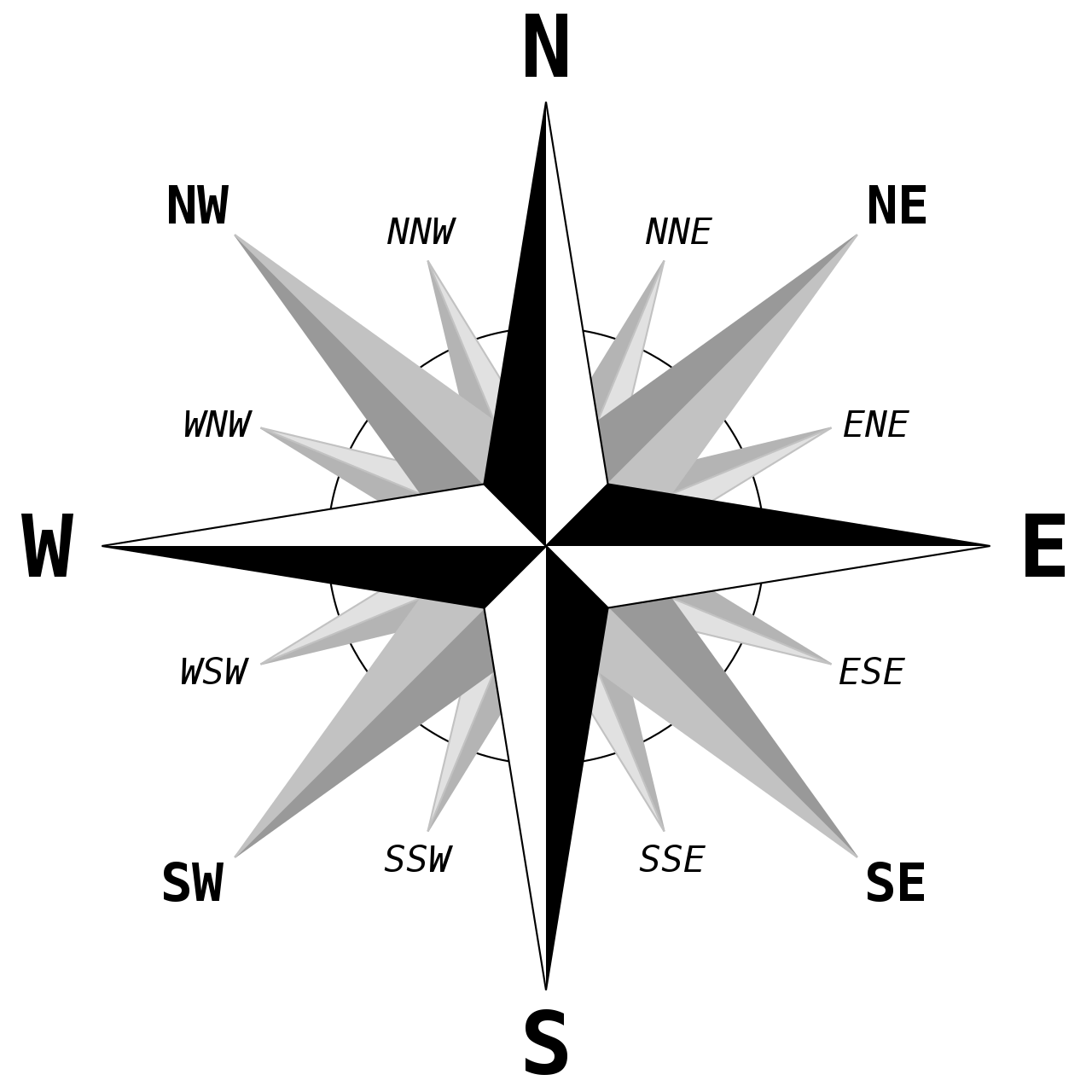
We can use cardinal directions to specify the direction of displacement vectors. These directions can be described by a compass rose. The compass rose given in Figure 11.7.1 is an example of a sixteen point compass rose. Directions of the form ESE are read as “east-southeast” and point in the direction halfway between east and southeast.
A sixteen-point star shown with the point going up labeled N, the point going directly right labeled E, the point going down labeled S, and the point going left labeled W. The point going up and right is labeled NE, the point going down and right is labeled SE, the point going down and left is labeled SW, and the point going up and left is labeled NW. Between each of these points is eight points which are labeled (clockwise from the top) NNE, ENE, ESE, SSE, SSW, WSW, WNW, and NNW.
Below is a contour plot showing the elevations for a region of a nearby park. We will be referring to \(h(x,y)\) as the function of two variables that gives the elevation as a function of \(x\)-coordinate (location in the east-west or horizontal direction) and \(y\)-coordinates (location in the north-south or vertical direction).
A contour plot on which three points (\(A\text{,}\)\(B\text{,}\) and \(C\)) are marked. A compass is drawn in the bottom left of the plot and labels the up direction N, to the right is labeled E, down is labeled S, and to the left is labeled W. Many curves are drawn and labeled corresponding the height of a landscape at that point. Peaks in the landscape occur toward the top left and the middle on the right, as well as the bottom right corner of the region. A depression is in the middle top of the region.
Using the contour plot and treating the elevation as a multivariable function \(h(x,y)\text{,}\) state whether each of the following is positive, negative, or zero. Write a sentence to justify your reasoning.
Suppose you are standing at point \(B\text{.}\) Do you expect the elevation to increase, decrease, or remain constant if you take a step in the northeast direction? Write a sentence to explain your reasoning.
Suppose you are standing at point \(B\text{.}\) Do you expect the elevation to increase, decrease, or remain constant if you take a step in the southeast direction? Write a sentence to explain your reasoning.
Suppose you are standing at point \(A\text{.}\) Do you expect the elevation to increase, decrease, or remain constant if you take a step in the southwest direction? Write a sentence to explain your reasoning.
Suppose you are standing at point \(C\text{.}\) In what direction would you take a step to move in the steepest downhill direction? Write a sentence to explain your reasoning.
Suppose you are standing at point \(A\text{.}\) In what direction would you take a step to move in the steepest uphill direction? Write a sentence to explain your reasoning.
Suppose you are standing at point \(B\text{.}\) Rank the following directions in order of steepness (from most steep and uphill to level to most steep downhill): northeast, north, east, west, south
The Preview Activity demonstrates how visual information such as a contour plot or a surface plot can be helpful in determining information about how quickly the output of a function changes as its inputs change in different directions. In this section, we will focus on how to calculate this kind of directional derivative using algebraic or numerical representations of functions and relate this calculation to other ways we have described change for a function.
We begin by determining how to measure the rate of change for a function of two variables in a direction that is not parallel to one of the coordinate directions. We use the classic calculus approach to set up this measurement: approximate the measurement, quantify how the approximation changes on a smaller scale, and finally use a limit to find the value. To measure the rate of change in the output of a function, we use a difference quotient:
\begin{equation*}
\text{rate of change} = \frac{\text{change in output}}{\text{change in input}}\text{.}
\end{equation*}
Let \(f\) be a function of the variables \(x\) and \(y\text{.}\) We wish to measure the rate of change of \(f\) at the base point \((x_0,y_0)\) in the direction of the vector \(\langle a,b\rangle\text{.}\) To do this, we write the difference quotient using the points \((x_0+a,y_0+b)\) and \((x_0,y_0\)):
The denominator comes from using the distance formula to measure the change in the input as distance in the \(xy\)-plane. Figure 11.7.2 shows the plot of a surface given by \(z=f(x,y)\) with the points used in the difference quotient labeled.
A three dimensional plot of a curved surface shown in gray above a set of axes labeled \(x\text{,}\)\(y\text{,}\) and \(z\text{.}\) An arrow is shown below the surface on the xy-plane in blue. This arrow is labeled with \(\langle a ,b \rangle\) and as “change in input” while pointing in the direction of the x and y axes. Line segments from the ends of the blue arrow to the surface are drawn in gray. From the two points where the gray segments intersect the surface, there are two red segments that move parallel to the xy-plane to the z-axis. The distance between where the two red line segments intersect the z-axis is shown with red arrows and labeled as “change in output”.
The difference quotient above is the first step in the classic calculus approach and provides a good start to approximating the rate of change for the output of \(f\) in the direction \(\langle a,b\rangle\text{.}\) However, it is not clear how this approximation changes when we look at smaller scales. Specifically, we need to look at what happens to this approximation as we shrink the step size \(\sqrt{a^2+b^2}\) to \(0\) while maintaining the same direction of change. In order to maintain our direction and look at smaller step sizes, we must separate the length of the vector \(\langle a,b \rangle \) from its direction. To do this, we use the unit vector in the direction of \(\langle a,b \rangle\text{.}\)
Let \(\vu=\langle u_1,u_2\rangle \) be the unit vector in the same direction as \(\langle a,b \rangle\text{.}\) Vectors in the same direction as \(\langle a,b \rangle\) can be written in the form \(t \langle u_1,u_2\rangle\text{,}\) where \(t\) is the step size and \(\vu=\langle u_1,u_2\rangle \) is the unit vector. Taking a step of length \(t\) in the direction \(\langle u_1,u_2 \rangle\text{,}\) the difference quotient can be written as
We will look at how this difference quotient changes at smaller scales, i.e., when the step size \(t\) gets smaller. This accomplishes the second step of the classic calculus approach because it quantifyies how the approximation works on smaller scales. We can now take the limit as \(t \to 0\) to define the directional derivative.
Let \(f(x,y)\) be a function of two variables. The derivative of \(f\) at the point \((x,y)\) in the direction of the unit vector \(\vu = \langle u_1, u_2 \rangle\) is denoted \(D_{\vu}f(x,y)\) and is given by
The notation \(D_{\vu}f(x,y)\) can also be read as “the directional derivative of \(f\) in the direction \(\vu\) at the point \((x,y)\text{.}\)” While this may seem like a mouthful, each piece of this phrase is necessary to specify a directional derivative: we must specify the function, the location at which to measure the rate of change, and the direction in which the inputs change. When we evaluate the directional derivative \(D_{\vu} f(x,y)\) at a point \((x_0, y_0)\text{,}\) the result \(D_{\vu} f(x_0,y_0)\) tells us the instantaneous rate at which \(f\) changes at \((x_0, y_0)\) per unit increase in the direction of the vector \(\vu\text{.}\)
We can connect equation (11.7.1) to our work on traces earlier in this chapter. When initially exploring surface plots, we simplified our approach by looking at slices that were parallel to one of the coordinate axes, obtained by holding the other input variable constant. This allowed us to use ideas from single-variable calculus to understand more about the surface and to motivate the definitions of partial derivatives. Similarly, we can cut the surface in the \(\langle u_1,u_2\rangle \) direction through the base point and then think about the directional derivative as a single-variable calculus problem. In particular, we can parameterize the trace along the surface by noticing our inputs correspond to the line in the xy-plane given by \(\langle x_0+ u_1 t, y_0 + u_2 t\rangle\text{,}\) which is shown in red on Figure 11.7.4.
A three dimensional plot of a curved surface shown in gray above a set of axes labeled \(x\text{,}\)\(y\text{,}\) and \(z\text{.}\) The gray surface decreases as either x or y is increased from a maximum near the z-axis. An arrow is shown below the surface on the xy-plane in red. A line segment is shown in red on the xy-plane in same direction as the arrow and extends past the end of the arrow. This arrow is labeled with \(\langle u_1,u_2 \rangle\) while pointing in the direction of the x and y axes. A blue plane is shown extending from the red line segment parallel to the z-axis, through the surface. The curve along the surface that is above the red segment and is the intersection between the curved surface and the blue plane is drawn in blue.
When \(t=0\text{,}\) the location is \((x_0,y_0)\text{.}\) The trace along the surface is given by \(\vr(t)=\langle x_0+ u_1 t, y_0 + u_2 t , f(x_0+ u_1 t, y_0 + u_2 t) \rangle\text{.}\) This trace is shown in blue in Figure 11.7.4. We can also plot the trace of this surface in the direction of \(\langle u_1,u_2 \rangle\) as a function of \(t\) using a two-dimensional plot. This plot is shown in Figure 11.7.5. We can visualize the directional derivative as the slope of a tangent line at the base point. This tangent line is drawn in black on Figure 11.7.5. The scalar \(D_{\vu} f(x_0,y_0)\) tells us the slope of the line tangent to the surface in the direction of \(\vu\) at the point \((x_0,y_0,f(x_0,y_0))\text{.}\)
A two-dimensional plot with the vertical axis labeled \(f(x_0+tu_1,y_0+tu_2)\) and the horizontal axis labeled \(t\text{.}\) A curve in blue, that starts between the second and third grid lines vertically, decreases until just after the third grid line on the horizontal axis. The tangent line to the curve at the left most point is shown and moves down but more to the right than down.
Figure11.7.5.A plot of the trace of \(f\) along the direction \(\langle u_1,u_2\rangle\) with tangent line drawn at point corresponding to \((x_0,y_0)\)
Subsection11.7.3Efficiently Computing the Directional Derivative
We want to find a way to evaluate directional derivatives without resorting to evaluating the limit definition in equation (11.7.1) every time. We will look at this algebraic approach from two perspectives. First, we will use the chain rule from Section 11.6 to define a simple algebraic rule which will allow us to efficiently calculate directional derivatives. Second, we will use the linearization of a locally linear function to compute directional derivatives.
We are interested in the instantaneous rate of change of \(f\) at a point \((x_0,y_0)\) in the direction of a unit vector \(\vu = \langle u_1, u_2 \rangle\text{.}\) In particular, the input variables \(x\) and \(y\) are changing according to
\begin{equation*}
x = x_0 + u_1t \quad \text{ and } \quad y = y_0 + u_2t\text{.}
\end{equation*}
A trace along the surface in the direction of \(\langle u_1,u_2\rangle\) is given by \(\vr(t)=\langle x_0+ u_1 t, y_0 + u_2 t , f(x_0+ u_1 t, y_0 + u_2 t) \rangle\text{.}\) Observe that \(\frac{dx}{dt} = u_1\) and \(\frac{dy}{dt} = u_2\) for all values of \(t\text{.}\) Since \(\vu\) is a unit vector in the \(xy\)-plane, a unit change in the parameter \(t\) corresponds to moving one unit in the \(\vu\) direction. This allows us to use the multivariable chain rule to calculate the directional derivative as a measure of the instantaneous rate of change of \(f\) in the direction \(\vu\text{.}\)
The output of \(f\) along the given direction can be written as a composition of functions, \(f(t)=f(\vr(t))=f(x(t), y(t))\text{,}\) which means we can apply the multivariable chain rule:
Given a differentiable function \(f = f(x,y)\) and a unit vector \(\vu = \langle u_1, u_2 \rangle\text{,}\) the directional derivative \(D_{\vu}f(x,y)\) can be computed by
To use equation (11.7.2), we must have a unit vector \(\vu = \langle u_1, u_2 \rangle\) in the direction of motion. In the event that we have a direction prescribed by a non-unit vector, we must first scale the vector to have length 1.
We will look at an example that is algebraically and geometrically simple but allows us to use Theorem 11.7.6. We will consider the rate of change for the function \(f(x,y)=2.5-\frac{(x-1)^2}{2}-\frac{(y+1)^2}{9}\) at the input point \((2,2)\) in several directions. Because \(f(2,2)=2.5-\frac{(2-1)^2}{2}-\frac{(2-2)^2}{9}=2.5-0.5-1=1\text{,}\) this point lies on the level curve with value \(1\) as shown in Figure 11.7.8.
A contour plot that shows several concentric ellipses around the point (1,-1). The point \((2,2)\) is highlighted in black and an arrow pointing left and up from this point is shown in red.
We will compute the directional derivative of \(f\) at the point \((2,2)\) in the direction of \(\langle-2,-1\rangle\text{.}\) Since \(\langle-2,1\rangle\) is not a unit vector, we use \(\vu=\frac{1}{\sqrt{5}}\langle -2,1\rangle\) as the unit vector in this direction. To use equation (11.7.2), we will need the partial derivatives of \(f\text{:}\)
\begin{equation*}
f_x= -\frac{2(x-1)}{2} \quad \text{ and } \quad f_y=-\frac{2(y+1)}{9}
\end{equation*}
At \((2,2)\text{,}\) we have \(f_x(2,2)=-1\) and \(f_y(2,2)=-\frac{2}{3}\text{.}\) By equation (11.7.2), the directional derivative of \(f\) at \((2,2)\) in the direction \(\vu\) is
We can interpret this as saying that for a small step in the direction of \(\vu\) at \((2,2)\text{,}\) we would expect the output of \(f\) to increase by \(\frac{4}{3\sqrt{5}}\) times the step size.
This may be a bit difficult to see based on the contour plot in Figure 11.7.8. However, the surface plot combined with a plot of the path of inputs in the direction \(\vu\) gives a better visualization. Figure 11.7.9 shows a surface plot of \(z=f(x,y)\) with the trace in the \(\vu\)-direction shown in blue and the direction vector \(\vu\) shown in red on the \(xy\)-plane. The black line segment shows how \(Df_\vu(2,2)\) is positive because the \(z\)-coordinate of this tangent line increases as we move away from \((2,2)\) in the \(\vu\)-direction.
A three dimensional plot of a curved surface shown in gray above a set of axes labeled \(x\text{,}\)\(y\text{,}\) and \(z\text{.}\) The gray surface decreases as you move away from from a maximum near the z-axis. An arrow is shown below the surface on the xy-plane in red and points in the direction of the x and y axes. A gray segment is drawn from the beginning point of the red arrow, parallel to the z-axis, up to the surface. A point where the gray segment intersects the surface his highlighted. A blue plane is shown extending from the red arrow parallel to the z-axis, through the surface. The curve along the surface that is above the red segment and is the intersection between the curved surface and the blue plane is drawn in blue. This blue curve initially increases in z then decreases. The line segment that begins at the highlighted point and is tangent to the blue curve is shown in black.
Remember that the directional derivative is a local measurement and only applies in a small neighborhood of a point and only in the direction \(\vu\text{.}\) In other words, \(Df_\vu(2,2)\) does not describe the the rate of change at other points along the blue curve, only the rate of change along the blue curve for a small step away from our base point in the red direction. With plots like Figure 11.7.8, you may be tempted to use information far away from the point of interest to try to figure out the rate of change. However, like most calculus measurements, we must only use plots to provide information on what is happening near a specific point.
If we compute \(Df_\vj(2,2)\text{,}\) the rate of change for the output of \(f\) in the direction \(\vj=\langle 0,1\rangle\) at \((2,2)\text{,}\) using equation (11.7.2), then we have
Figure 11.7.10 allows you to adjust the direction of the trace shown. By default, it shows the direction vector \(\vj\text{,}\) the cooresponding trace, and tangent line to the surface in the \(\vj\) direction. Use the slider at the top of Figure 11.7.10 to change the direction in which you want to evaluate the directional derivative. As you do so, examine how the steepness of the black tangent segment varies depending on the direction.
An interactive three dimensional plot of a curved surface shown in gray above a set of axes labeled \(x\text{,}\)\(y\text{,}\) and \(z\text{.}\) The gray surface decreases as you move away from from a maximum near the z-axis. A slider at the top of the figure changes the direction of an arrow shown below the surface on the xy-plane in red. A gray segment is drawn from the beginning point of the red arrow, parallel to the z-axis, up to the surface. A point where the gray segment intersects the surface his highlighted. A blue plane is shown extending from the red arrow parallel to the z-axis, through the surface. The curve along the surface that is above the red segment and is the intersection between the curved surface and the blue plane is drawn in blue. As the direction of the red arrow changes the profile of the blue curve changes according to the shape of the surface in the given direction.
Use equation (11.7.2) to determine \(D_{\vi} f(x,y)\) and \(D_{\vj} f(x,y)\text{.}\) Write a couple of sentences to describe what familiar functions \(D_{\vi} f\) and \(D_{\vj} f\) are.
Use equation (11.7.2) to find the derivative of \(f\) in the direction of the vector \(\vv = \langle -2, -3 \rangle\) at the point \((1,-1)\text{.}\) Write a couple of sentences to explain why this result is different from your answer to the previous two tasks, even though the direction vectors are parallel.
Equation (11.7.2) arose through consideration of the definition for the directional derivative as a composition of functions and application of the chain rule. When considering multivariable functions that are locally linear, recall that we can evaluate the limit of such a function near a point by analyzing the linearization or tangent plane. On a small scale, there is virtually no difference between the locally linear function and the linearization as demonstrated by Figure 11.5.1.
The equation of the plane tangent to the graph of \(f\) at the point \((x_0,y_0,f(x_0,y_0))\) is
\begin{equation*}
z = f(x_0,y_0) + f_x(x_0,y_0)(x-x_0) + f_y(x_0,y_0)(y-y_0)\text{.}
\end{equation*}
If \(f\) is a locally linear function, then the directional derivative \(D_{\vu}f(x_0,y_0)\) is the same as the rate of change along the tangent plane in the direction of \(\vu\text{.}\) This is convenient because on the tangent plane, the rate of change is the same regardless of step size, a fact that is not true on the original surface \(z=f(x,y)\text{.}\) We now consider the quotient
We have used the chain rule and linearization to see see that the instantaneous rate of change a function \(f = f(x,y)\) in the direction of a unit vector \(\vu = \langle u_1, u_2 \rangle\) is given by
You may recognize the form of (11.7.3) as being similar to a dot product. We can also view this equation as stating that the rate of change along the linearization in a given direction can be expressed as a linear combination of the rates of change in the coordinate directions by using partial derivatives with the weight of each partial derivative specified by the components of the unit vector \(\vu\text{.}\)
We can think about equation (11.7.3) in a way that will have geometric meaning related to the dot product. The directional derivative \(D_{\vu}f(x_0,y_0)\) is the dot product of \(\left\langle f_x(x_0,y_0), f_y(x_0,y_0) \right\rangle\) and \(\vu=\langle u_1,u_2\rangle\text{.}\) Notice that the vector \(\left\langle f_x(x_0,y_0), f_y(x_0,y_0) \right\rangle\) comes from simple calculations that tell us how the function \(f\) is changing near the input \((x_0,y_0)\text{.}\)
A contour plot with the horizontal and vertical axes going from -4 to 4. A pair of intersecting lines going from the top left to the bottom right and from the bottom left to the top right are labeled 0. Eight sets of hyperbolas with asymptotes given by the intersecting lines are drawn centered at the origin. The hyperbolas that are opening to the right and left are labeled from 1 to 4 as they step away from the origin. The hyperbolas that are opening to the top[ and bottom are labeled from -1 to -4 as they step away from the origin.
For each of the following points \((x_0,y_0)\text{,}\) evaluate the gradient \(\nabla f(x_0,y_0)\) and sketch the gradient vector with its tail at \((x_0,y_0)\text{.}\) Some of the vectors are too long to fit onto the plot. To draw them to scale, you should scale each vector by a factor of \(1/2\text{.}\)
Does the output of \(f\) increase or decrease in the direction of \(\nabla f(x_0,y_0)\text{?}\) Use examples from the points above to write a couple of sentences that justify your answer.
You may wish to think about the contour plot as a topographical map and whether your elevation would increase or decrease if you took a step in the direction of the gradient.
Because \(\nabla f(x_0,y_0)\) is a vector, we can consider its direction and length separately. The next subsection discusses the information conveyed by these geometric aspects about the behavior of \(f\) near \((x_0,y_0)\text{.}\)
Key Idea 11.7.12 shows how we can separate the directional derivative of a function of two variables into two separate parts: the gradient vector evaluated at the point of interest and the unit vector in the direction we want to change the inputs of the function. Recall from equation (9.3.1) that the dot product of two vectors depends on the lengths of the vectors and the angle between the vectors. If \(\theta\) is the angle between \(\nabla f(x_0,y_0)\) and \(\vu\) (where \(\vu\) is a unit vector), then combining (11.7.4) and (9.3.1) gives
Remember that \(\vecmag{\vu}=1\) because \(\vu\) is a unit vector. Hence, the directional derivative is the length of the gradient vector times the cosine of the angle between \(\nabla f(x_0,y_0)\) and \(\vu\text{:}\)
A two dimensional plot with the horizontal axis labeled x and vertical axis labeled y. A red highlighted point is shown in the first quadrant and is labeled \((x_0,y_0)\text{.}\) Two arrows are drawn from the highlighted point. The first vector moves from the red highlighted point more to the left than up and is labeled \(\vec{u}\text{.}\) The second arrow is longer and moves from the red point more up than to the right. The second arrow is labeled \(D_{\vu} f(x_0,y_0)\text{.}\) The right angle between these arrows is shown with a circular arc and is labeled \(\theta\text{.}\)
A two dimensional plot with the horizontal axis labeled x and vertical axis labeled y. A red highlighted point is shown in the first quadrant and is labeled \((x_0,y_0)\text{.}\) Two arrows are drawn from the highlighted point. The first vector moves from the red highlighted point more up than left and is labeled \(\vec{u}\text{.}\) The second arrow is longer and moves from the red point more up than to the right. The second arrow is labeled \(D_{\vu} f(x_0,y_0)\text{.}\) The acute angle between these arrows is shown with a circular arc and is labeled \(\theta\text{.}\)
A two dimensional plot with the horizontal axis labeled x and vertical axis labeled y. A red highlighted point is shown in the first quadrant and is labeled \((x_0,y_0)\text{.}\) Two arrows are drawn from the highlighted point. The first vector moves from the red highlighted point directly left and is labeled \(\vec{u}\text{.}\) The second arrow is longer and moves from the red point more up than to the right. The second arrow is labeled \(D_{\vu} f(x_0,y_0)\text{.}\) The obtuse angle between these arrows is shown with a circular arc and is labeled \(\theta\text{.}\)
Because the magnitude of a vector is always non-negative, the sign of a directional derivative depends on \(\cos(\theta)\text{.}\)Figure 11.7.14 graphically shows examples of the following statements (from left to right):
If the angle between the gradient and \(\vu\) is a right angle, then the directional derivative is zero.
The first statement explains why the gradient is perpendicular to the level curve through the point of interest. Because a level curve is the set of points for which the function has a particular output value, the output will not change along the level curve. Thus, the directional derivative in a direction tangent to the level curve must be zero. We can expand this explanation to the other statements as well. The output of \(f\) increases in any direction that makes an acute angle with the gradient vector and the output of \(f\) decreases in any direction that makes an obtuse angle with the gradient.
For this activity, we will look at the value of the directional derivative for temperature as a function of location. When looking at a plot of thermoclines (locations with the same temperature), you notice that your town is exactly on the thermocline labeled as 70 degrees, shown as the point \(P\) on Figure 11.7.15
A two dimensional plot with a compass shown in the top left. The compass labels up N, to the right E, down S and to the left W. A curve extends from the bottom left to the top right of the region, through a point labeled \(P\) in the center of the plot. The region above and to the left of this curve is labeled “60s” and the region below and to the right of the curve is labeled “70s”. An arrow is drawn from the highlighted point to the right and down. This arrow is perpendicular to the curve at the highlighted point.
Write a few sentences about why the gradient at \(P\) goes in the southeast direction and not the northwest (which is also perpendicular to the thermocline/ level curve at \(P\)).
Draw a vector in each of the following directions starting at \(P\) and state whether the directional derivative will be positive/negative/0 in each of these directions. You should write a couple of sentences for each direction vector about how the sign of the directional derivative is related to the angle between the direction and the gradient vectors.
Explain what direction you would need to move in to have the greatest positive rate of change for the temperature. Write a couple of sentences to relate your answer to the gradient using Equation (11.7.5).
All of these questions can be answered by considering equation (11.7.5). Because the length of the gradient vector does not change when changing direction, the \(\cos(\theta)\) factor tells us when we have the maximum and minimum values. Because of how we define the angle between vectors, we only need to consider values of \(\theta\) between 0 and \(\pi\text{.}\) Therefore, the largest value of the directional derivative occurs when \(\theta=0\) and \(\cos(\theta)\) attains its maximum value of \(1\text{.}\) This means that when the direction vector \(\vu\) is in the same direction as the gradient, the directional derivative is maximized. Furthermore, the largest value of the directional derivative is the length of the gradient. In equation form, we can express that if \(\vu\) is in the same direction as \(\nabla f(x_0,y_0)\text{,}\) then
By a parallel argument, the smallest (or most negative) value the directional derivative can take is when \(\theta=\pi\text{.}\) In this case, the direction vector is in the opposite direction of the gradient vector. Thus if \(\theta=\pi\text{,}\) then
The gradient \(\nabla f(x_0,y_0)\) points in the direction of greatest rate of increase for \(f\) at \((x_0,y_0)\text{,}\) and the instantaneous rate of change of \(f\) in that direction is the length of the gradient vector.
If \(\vu = \frac{1}{\vecmag{\nabla f(x_0,y_0)}} \nabla f(x_0,y_0)\text{,}\) then \(\vu\) is a unit vector in the direction of greatest increase of \(f\) at \((x_0,y_0)\text{,}\) and \(D_{\vu} f(x_0,y_0) = \vecmag{\nabla f(x_0,y_0)}\text{.}\)
The gradient \(\nabla f(x_0,y_0)\) points in the opposite direction of greatest rate of decrease for \(f\) at \((x_0,y_0)\text{,}\) and the instantaneous rate of change of \(f\) in that direction is the length of the gradient vector times \(-1\text{.}\)
If \(\vu = -\frac{1}{\vecmag{\nabla f(x_0,y_0)}} \nabla f(x_0,y_0)\text{,}\) then \(\vu\) is a unit vector in the direction of greatest decrease of \(f\) at \((x_0,y_0)\text{,}\) and \(D_{\vu} f(x_0,y_0) = -\vecmag{\nabla f(x_0,y_0)}\text{.}\)
We will look algebraically calculating and explaining the vector properties of the gradient using the function \(f(x,y)=xy-2y^2+\frac{x^2}{2}+2y-x\) at the input \((1,1)\text{.}\)
What direction will correspond to the greatest rate of increase for \(f\) at the input \((1,1)\text{?}\) Find the value of the directional derivative in this direction.
Exercises 11–13 look at how the directional derivative changes as a function of the direction used or of the point where the directional derivative is being evaluated.
The gradient has many natural applications. For example, situations often arise where we are interested in knowing the direction in which a function is increasing or decreasing most rapidly. This type of question is natural when constructing a road through the mountains or planning the flow of water across a landscape. In the next activity, we examine how the gradient can help with navigation to the top of a mountain in foggy conditions.
This activity considers directional derivatives and gradients for a function that measures elevation. Suppose you are hiking in a foggy park and can only see a few feet in front of you. There is nothing blocking you from walking in any particular direction, but because of the fog you cannot see where the highest point on the mountain is. You want to try to find the top of the mountain, but you don’t have a map, trail, or line of sight to other landmarks. You do have a compass, which works in the fog. This allows you to identify the cardinal directions.
In order to use calculational tools from multivariable calculus, you overlay an \(xy\)-coordinate system on the park. The \(x\)-coordinate measures east/west location, with eastward movement associated with increasing \(x\)-values. The \(y\)-coordinate measures north/south location, with northward movement associated with increasing \(y\)-values. The elevation in meters above sea level of the park’s terrain at the location \((x,y)\) is given by a function \(h(x,y)\text{.}\)
Let \(P_1\) be your current location in the foggy park. You use your compass to find the east and north directions. At \(P_1\text{,}\) you find that the ground rises 1 meter per 50 meters traveled to the east and the ground rises 2.5 meters per 50 meters traveled to the north.
You decide to walk uphill from your location \(P_1\) in order to try to find the top of the mountain. After walking in the same direction for a while, you are at a point \(P_2\) and notice that you are no longer walking in the steepest direction. You again locate east and north and measure the steepness of the mountain in these directions. You find that the ground rises 1.5 meters per 75 meters traveled to the east and the ground goes down 0.5 meters per 100 meters traveled to the north.
Use this new information to calculate \(\nabla h (P_2)\text{,}\) find the uphill direction, and find how steep the mountain is in the uphill direction at \(P_2\text{.}\)
Suppose you continue this method of walking in the uphill direction for a while, finding the new uphill direction, and walking in the new uphill direction. Do you think you must eventually find the top of the mountain? How you will know that you have reached the top of the mountain? Remember that you can’t see very far in front of you. Write a few sentences to explain your reasoning.
The technique described in the previous activity has many applications related to maximizing or minimizing functions. For example, consider a two-dimensional version of how a heat-seeking missile might work. (This application is borrowed from United States Air Force Academy Department of Mathematical Sciences.) Suppose that the temperature surrounding a fighter jet can be modeled by the function \(T\) defined by
where \((x,y)\) is a point in the plane of the fighter jet and \(T(x,y)\) is measured in degrees Celsius. Some contours and gradients \(\nabla T\) are shown on the left in Figure 11.7.16.
A two dimensional plot with horizontal scale from 0 to 10 and vertical scale from 0 to 5. Concentric ellipses are shown centered at the point (5,2.5). A grid of gray vectors is shown such that each vector points in a direction perpendicular to the ellipses. The ellipses are labeled 10, 17, and 50 for the three closest to the center.
A two dimensional plot with horizontal scale from 0 to 10 and vertical scale from 0 to 5. Concentric ellipses are shown centered at the point (5,2.5). A grid of gray vectors is shown such that each vector points in a direction perpendicular to the ellipses. The ellipses are labeled 10, 17, and 50 for the three closest to the center. A red curve is shown from (2,4) to the center of the figure such that the red curve crosses each of the ellipses in a perpendicular direction.
A heat-seeking missile will always travel in the direction in which the temperature increases most rapidly; that is, it will always travel in the direction of the gradient \(\nabla T\text{.}\) If a missile is fired from the point \((2,4)\text{,}\) then its path will be that shown on the right in Figure 11.7.16.
This type strategy is sometimes called gradient ascent. The gradient decent method is used to find relative minimums for functions by taking steps in the direction opposite the gradient. Gradient decent methods are used extensively in economics and machine learning to find where the difference between predictions from a model and data are as small as possible (minimize error).
for those values of \(x\) and \(y\) for which the limit exists. In addition, \(D_{\vu}f(x,y)\) measures the slope of the graph of \(f\) when we move in the direction \(\vu\text{.}\) Alternatively, \(D_{\vu} f(x_0,y_0)\) measures the instantaneous rate of change of \(f\) in the direction \(\vu\) at \((x_0,y_0)\text{.}\)
At any point where the gradient is nonzero, the gradient is orthogonal to the contour through that point and points in the direction in which \(f\) increases most rapidly; moreover, the slope of \(f\) in this direction equals the length of the gradient \(\vecmag{\nabla f(x_0,y_0)}\text{.}\) Similarly, the direction opposite of the gradient is the direction of greatest decrease, and that rate of decrease is the negative length of the gradient.
Find the rate of change of the function \(f\) at the point (-1, 2,-4) in the direction \(\mathbf u = \langle 5/\sqrt{27}, 1/\sqrt{27}, 1/\sqrt{27} \rangle\text{.}\)
If \(f \left( x, y \right) = -2 x^{2} + 3 y^{2}\text{,}\) find the value of the directional derivative at the point \(\left( 4, 4 \right)\) in the direction given by the angle \(\theta = \frac{2 \pi}{6}\text{.}\)
Find the directional derivative of \(\displaystyle f(x,y,z) = 3xy+z^{2}\) at the point \((5,-2,1)\) in the direction of the maximum rate of change of \(f\text{.}\)
The temperature at a point (x,y,z) is given by \(\displaystyle
T(x,y,z) = 200e^{-x^2 -y^2/4 - z^2/9}\text{,}\) where \(T\) is measured in degrees Celsius and x,y, and z in meters. There are lots of places to make silly errors in this problem; just try to keep track of what needs to be a unit vector.
The concentration of salt in a fluid at \((x,y,z)\) is given by \(F(x,y,z) = x^{2}+3y^{4}+4x^{2}z^{2}\) mg/cm\({}^3\text{.}\) You are at the point \((1,1,-1)\text{.}\)
At a certain point on a heated metal plate, the greatest rate of temperature increase, 2 degrees Celsius per meter, is toward the northeast. If an object at this point moves directly north, at what rate is the temperature increasing?
The next three exercises consider how the directional derivative changes as a function of the direction used or of the point where the directional derivative is computed. The goal of these exercises is to understand the directional derivative as a geometric measurement using visually-based sense-making prompts in terms of the location and directions being used. In particular, Exercise 11 asks students to visually assess whether the directional derivative is positive/negative/zero at a few locations and directions. Exercise 12 fixes the location on a surface and steps students about how to construct a function that gives value of the directional derivative as a function of the direction. Exercise 13 examines the relationships between the value of the directional derivative and ideas like the slope of a secant line or dependence on the length of the direction vector. These exercises are adapted from materials developed by Rafael Martinez-Planell.
Draw a piece of the tangent line to the graph of \(f\) at the point \((2,-1,f(2,-1))\) which is in the direction \(\langle 1,1\rangle \text{.}\) The slope of the tangent line in the \(\langle 1,1\rangle \) direction is called the directional derivative of \(f\) at \((2,-1)\) in the \(\langle 1,1\rangle \) direction and is denoted \(D_{\langle 1,1\rangle} f (2,-1)\text{.}\)
On the \(xy\)-plane of (a new plot of) the figure below, draw the direction vector \(\langle -\frac{1}{2},3\rangle \) starting at the point \((2,-1)\text{.}\)
Draw a piece of the tangent line to the graph of \(f\) at the point \((2,-1,f(2,-1))\) which is in the direction \(\langle -\frac{1}{2},3 \rangle \text{.}\) The slope of the tangent line in the \(\langle -\frac{1}{2},3 \rangle \) direction is called the directional derivative of \(f\) at \((2,-1)\) in the \(\langle -\frac{1}{2},3 \rangle \) direction and is denoted \(D_{\langle -\frac{1}{2},3 \rangle} f (2,-1)\text{.}\)
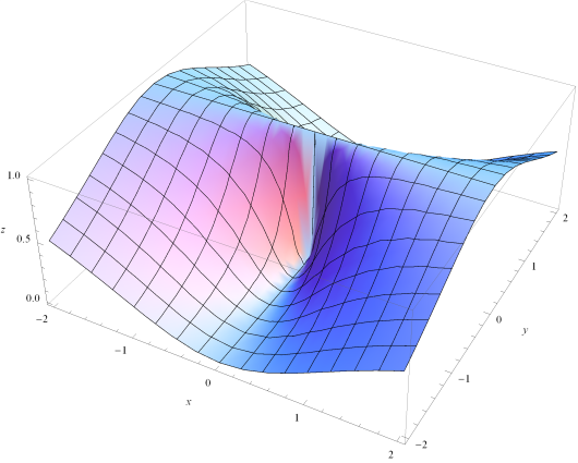
Let \(f\) be the function whose graph appears in Figure 11.7.17. For each value of \(t\) the vector \(\langle \cos(t),\sin(t)\rangle \) is a direction vector. The value of \(D(t)=D_{\langle \cos(t),\sin(t)\rangle} f (1,-1)\) a scalar.
Draw the graph of \(y=D(t)\) for values of \(t\) in the interval \([0,2\pi]\text{.}\) You should think about how the value of \(D(t)\) changes between the values you considered above to help you draw the graph of \(D(t)\text{.}\) Your graph doesn’t have to have exact values but should correctly identify where \(D(t)\) is positive, negative, and zero.
Draw the graph of \(y=G(t)=D_{\langle 1,1 \rangle} f (t,-t)\) for values of \(t\) in the interval \((0,2]\text{.}\) You should probably go through the same process you did above of looking at what \(G(t)\) will be for a few values of \(t\) between 0 and 2, then think about how \(G(t)\) will vary for values in between. The function \(G(t)\) is different than \(D(t)\text{.}\)
The graph of \(z=f(x,y)\) is as given below. In this problem, use geometric arguments to justify your answers.
Draw the line segment that goes from \((1,-1,f(1,-1))\) to \((2,0,f(2,0))\text{.}\) How does the slope of this line segment in that direction compare (smaller, equal, larger) with the value of \(D_{\langle 1,1 \rangle} f (1,-1)\text{?}\)
Which is closer to \(D_{\langle 1,1 \rangle} f (1,-1)\text{,}\) the slope of the line segment that goes from \((1,-1,f(1,-1))\) to \((2,0,f(0,2))\) or the slope of the line segment that goes from \((1,-1,f(1,-1))\) to \((1.01,-0.99,f(1.01,-0.99))\text{?}\) Explain your answer.
Let \(E(x,y) = \frac{100}{1+(x-5)^2 + 4(y-2.5)^2}\) represent the elevation on a land mass at location \((x,y)\text{.}\) Suppose that \(E\text{,}\)\(x\text{,}\) and \(y\) are all measured in meters.
Let \(\vu\) be a unit vector in the direction of \(\langle -4,3 \rangle\text{.}\) Determine \(D_{\vu} E(3,4)\text{.}\) What is the practical meaning of \(D_{\vu} E(3,4)\) and what are its units?
Find the direction of greatest increase in \(f\) at the point \((1,2)\text{.}\) Explain. A graph of the surface defined by \(f\) is shown at left in Figure 11.7.18. Illustrate this direction on the surface.
The properties of the gradient that we have observed for functions of two variables also hold for functions of more variables. In this problem, we consider a situation where there are three independent variables. Suppose that the temperature in a region of space is described by
and that you are standing at the point \((1,2,-1)\text{.}\)
Find the instantaneous rate of change of the temperature in the direction of \(\vv=\langle 0, 1, 2\rangle\) at the point \((1,2,-1)\text{.}\) Remember that you should first find a unit vector in the direction of \(\vv\text{.}\)