Active Calculus - Multivariable

The functions you are most familiar with have the form \(y=f(x)\) where \(x\) is the input or domain variable and \(y\) is viewed as the output variable. The graphs of these functions are plotted on a coordinate plane with the input expressed in terms of the horizontal coordinate and the output as the vertical coordinate. The following preview activity asks you to recall some algebraic and geometric ideas from before your single variable calculus course.

As you read in the introduction to this chapter, we will need to expand beyond the idea of measuring change involving expressions with one number as an input or output. One of the new kinds of functions we will examine is of the form \(z=g(x,y)\text{,}\) where the input is an ordered pair, \((x,y)\text{,}\) and the output of the function \(g\) is the real number \(z\text{.}\) In order to graph such a function, we will need to represent the basic ideas of coordinates and functions in a more general setting to accommodate more dimensions.

The tasks in Preview Activity 9.1.1 connect ideas used in coordinates and graphing for two dimensions to specific measurements. We will use these connections to build useful tools for three or more dimensions. In the rest of this section, we will define the measurements for coordinates and basic measurements in three dimensions.

We let \(\R^2\) denote the set of all ordered pairs of real numbers in the plane (two copies of the real number system) and let \(\R^3\) represent the set of all ordered triples of real numbers, which constitutes three-dimensional space. For example, \((1,\pi)\) is in \(\R^2\) and \((-e^2,\frac{\sqrt{7}}{4},0)\) is in \(\R^3\text{,}\) but \((\ln(3),2i)\) is not in \(\R^2\) because the second coordinate, \(2i\text{,}\) is an imaginary number and not a real number.

To plot points in three-dimensional space, we will set up a coordinate system with three mutually perpendicular axes—the \(x\)-axis, the \(y\)-axis, and the \(z\)-axis (called the coordinate axes). There are essentially two different ways we could set up a 3D coordinate system, as shown in Figure 9.1.4, which depicts only the positive portions of the axes. Thus, before we can proceed, we need to establish a convention.

The distinction between these two figures is subtle, but important. In the coordinate system shown in Figure 9.1.4.(a), imagine that you are sitting on the positive \(z\)-axis next to the label “\(z\text{.}\)” Looking down at the \(x\)- and \(y\)-axes, you see that the \(y\)-axis is obtained by rotating the \(x\)-axis by \(90^\circ\) in the clockwise direction. Again sitting on the positive \(z\)-axis in the coordinate system at right in Figure 9.1.4.(b), you see that the \(y\)-axis is obtained by rotating the \(x\)-axis by \(90^\circ\) in the counterclockwise direction.

We call the coordinate system in Figure 9.1.4.(b) a right-hand system; if we point the index finger of our right hand along the positive \(x\)-axis and our middle finger along the positive \(y\)-axis, then our thumb points in the direction of the positive \(z\)-axis. Following mathematical conventions, we choose to use a right-hand system throughout this book.

We let \(\R^2\) denote the set of all ordered pairs of real numbers in the plane (two copies of the real number system) and let \(\R^3\) represent the set of all ordered triples of real numbers (which constitutes three-space). For example, \((1,\pi)\) is in \(\R^2\) and \((-e^2,\frac{\sqrt{7}}{4},0)\) is in \(\R^3\text{,}\) but \((\ln(3),2i)\) is not in \(\R^2\) because the second coordinate is not a real number because \(2i\) is imaginary.

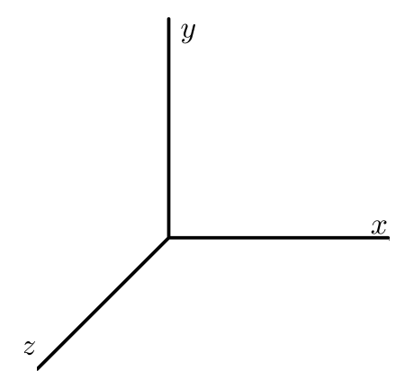
In other disciplines or settings you may see the \(y\)-axis as being oriented vertically with the \(x\)-axis going left/right and the \(z\)-axis going in and out of the page like in the figure below. This orientation may be useful for you because you can think of the traditional orientation of the \(xy\)-plane (when drawn on paper) with the positive \(z\)-axis coming out of the page.

Now that we have established how our axes will be defined, we can use these axes to define how to measure coordinates and make a few basic graphs.

In two dimensions, the horizontal coordinate was measured as the (perpendicular) distance to the vertical axis and the vertical coordinate was measured as the (perpendicular) distance to the horizontal axis. It is convenient to treat these measurements as signed distances with the measurement being positive when the point is above the given axis and negative when the measurement is below the given axis.

Figure 9.1.6 shows the measurement of coordinates for \(P\text{,}\) a point in the first quadrant, and \(Q\text{,}\) a point in the fourth quadrant. Notice that the coordinates \(a\text{,}\) \(b\text{,}\) and \(c\) will be positive because each of the segments used to measure the distance are above the other coordinate axis. The coordinate \(d\) will be negative because the segment used to measure the vertical distance to the \(x\)-axis is below the \(x\)-axis. This is what we mean when we say that the coordinate measurements are a signed distance: the distance specifies how far the point is from each axis, while the sign specifies whether that distance is above or below the axis.

In a three dimensional space, we need to pay attention to not just the axes but also the coordinate planes. Figure 9.1.7 shows how the \(xz\)-plane is the plane that contains the \(x\)- and \(z\)-axes. We can define the \(xy\)-plane as the plane that contain the \(x\)-and \(y\)-axes and the \(yz\)-plane as the plane that contain the \(y\)-and \(z\)-axes.

In Figure 9.1.7, you can click on the buttons to either show or hide each of the coordinate planes. You should explore and turn each of the coordinate planes on and pay attention to how each plane is oriented with respect to the different axes. Figure 9.1.7 is the first interactable 3D plot, so we will take a moment to talk about other important ways you should interact with figures like this.

A wonderful feature of a figure like Figure 9.1.7 is that you can rotate the figure, zoom in or out, and change the point from which the figure is viewed. These will be very helpful actions to try when looking at interactive 3D graphs because this will help you visualize the fullest version of these graphs. There are often parts of these 3D figures that are "behind" other elements or might make more sense to you if viewed from a different perspective. By giving you control over how the graph is viewed, you will have the ability to look at features in whatever way helps you make the most sense at the time. We will always try to have the first orientation shown in these types of figure be helpful, but we will always be a bit limited by showing a 3D figure in a 2D medium.

To rotate a 3D interactable figure, you should left click and hold somewhere on the figure. While holding, you can rotate the figure by moving the point where you clicked up/down/left right. Additionally, you can move the point you are viewing the graph from by right clicking and holding while moving the cursor up/down/left/right. On touchscreen devices, you will need to touch with two fingers to act as a right click. The arrow keys on a keyboard will also move the point at which the figure is being viewed from. You can also zoom in or out having your cursor over the 3D interactable figure and using the scroll wheel on a mouse or using pinching/expanding motions with two fingers on touchscreen devices. Take a few minutes to explore these actions on the figure below and pay attention to how each of these actions will change your view of the graph.

In many ways the coordinate planes in three dimensions are analogous to the axes in two dimensions. We will split up three-dimensional space based on whether a location is above or below different coordinate planes and we will measure coordinates in three dimensions as distances from the coordinate planes.

In two dimensions, the four regions that are separated by the coordinate axes are called quadrants and are typically labeled as in the plot below.

The coordinate planes will divide our three dimensional space up into eight regions, which we will call octants. The first octant is the part of \(\mathbb{R}^3\) that is in the positive \(x-\text{,}\) \(y-\text{,}\) and \(z-\)directions. You should rotate Figure 9.1.9 to see how there are eight regions that our 3D space is split into and how the orientation of the positive axis directions relates to the first octant.

The octants above the \(xy\)-plane are ordered just like the quadrants in two dimensions (when viewed looking down the \(z-\)axis) and octants 5 through 8 have the same relationships but are below the \(xy\)-plane. For example, octant 7 lies below quadrant III of the \(xy\)-plane. You can use the checkbox in Figure 9.1.9 to show the labels of the other octants.

The location of a point in a three-dimensional space is measured with three coordinates. The three-dimensional rectangular coordinates are measured as the signed distances to each of the coordinate planes. For example, the point \((1,-2,3)\) is shown in Figure 9.1.10.

When drawing points (or other plots) in three dimensions, it is often useful to draw segments or other features that are parallel to coordinate axes in order to help the viewer see the orientation and locations. For instance, we hope that you will find it easier to understand the location of the point \((1,-2,3)\) in Figure 9.1.10 because of the parallel structures shown on the plot.

In Figure 9.1.10 you should click on the box labeled “Show Segments” to turn of the colored line segments. You should notice how hard it is to understand where the point is located without turning the axes or having the colored line segments. You can rotate the figure with the point drawn without the segments and get some idea of where the point lies relative to the axes but this is a difficult visual task.

You should now click on the box labeled “Show Coordinate Planes” in Figure 9.1.10 to display the segments used to determine the coordinates in three dimensions as they are measured from the point to the coordinate planes. Most of our plots will not draw the coordinate planes. Framing the important measurements of your plot with structures that are parallel to the coordinate axes is a helpful way to make plots more easily understood.

If you select the “Show Segments” option and turn off the “Show Coordinate Planes” in Figure 9.1.10, you can see how it is easier to understand the location of the point \((1,-2,3)\) because of the parallel structures that are shown on the plot. In particular, you can see the \(x\)- and \(y\)-coordinates measured in the \(xy\)-plane with the \(z\)-coordinate extended up. The segments drawn in this plot are usually reasonable to add to a drawing done by hand as well. Remember that interacting with and exploring different features you notice in the three-dimensional plots is an important part of building your understanding.

At this point, we are ready to understand graphs of some simple equations in three dimensions. For example, in \(\R^2\text{,}\) the graphs of the equations \(x=a\) and \(y=b\text{,}\) where \(a\) and \(b\) are constants, are lines parallel to the coordinate axes. Remember that a graph of an equation is a plot of all points that satisfy this equation. This means that the graph of an equation is a visual representation of all locations whose coordinates will make the left side of your equation equal to the right side of the equation. The equation should give you a way to test whether a point is on the graph or not.

For instance, the graph of \(x=2\) in two dimensions will be a vertical line with \(x\)-intercept of 2, because the points of the form \((2,y)\) satisfy the equation \(x=2\) (for any choice of \(y \in \mathbb{R}\)) as shown in Figure 9.1.11. In the next activity we consider the three-dimensional analogs of these kinds equations.

Activity 9.1.3 illustrates that equations where one of the rectangular coordinates is held constant lead to planes parallel to the coordinate planes. When we make the constant 0, we get the coordinate planes themselves . The \(xy\)-plane satisfies \(z=0\text{,}\) the \(xz\)-plane satisfies \(y=0\text{,}\) and the \(yz\)-plane satisfies \(x=0\) (see Figure 9.1.7). Planes of the form \(x=a\text{,}\) \(y=b\text{,}\) \(z=c\) are called fundamental planes are useful in understanding and building structures in three dimensions. You can see how the intersection of fundamental planes \(x=1\text{,}\) \(y=-2\text{,}\) and \(z=3\) corresponds to the point \((1,-2,3)\) in Figure 9.1.12. As always, you should rotate and change the viewpoint of the figure to make sure you understand how each fundamental plane and the point \(P\) are oriented relative to the axes.

In a plot like Figure 9.1.3, you see a grid that helps measure coordinates of points in 2D. In Figure 9.1.13 you can look at how a different number of fundamental planes forming a grid looks. You can use the slider to increase or decrease the number of fundamental planes displayed in the grid. When you have more than one plane in each direction there will be a lot of visual clutter and very hard to distinguish fine features, especially something in the middle of the plot. Contrast this to how helpful the grid in Figure 9.1.15 is.

We conclude this section by using our knowledge of how to measure straight-line distance in \(\R^2\) to find a formula for distance in three dimensions. On a related note, we define a circle in \(\R^2\) as the set of all points equidistant from a fixed point. In \(\R^3\text{,}\) we call the set of all points equidistant from a fixed point a sphere. To find the equation of a sphere, we need to understand how to calculate the distance between two points in three-space, and we explore this idea in the next activity.

The method used in Activity 9.1.4 does not depend on anything but the coordinates between the two points, so we can use the last result to measure the distance between any two points in \(\mathbb{R}^3\text{.}\)

As Activity 9.1.4 showed, the distance in two or three (or more!) dimensions depends on the change in each coordinate from one point to the other. Note that the distance does not depend on whether we consider \(P\) to \(Q\) or \(Q\) to \(P\text{.}\)

Squaring both sides, we come to the standard equation for a sphere.