It is very rare to have applied or theoretical problems that apply to a rectangular region, so we would like to extend the idea of using iterated integrals to evaluate non-rectangular regions; we explore one such example in the following preview activity.
A tetrahedron is a three-dimensional figure with four faces, each of which is a triangle. A picture of the tetrahedron \(T\) with vertices \((0,0,0)\text{,}\)\((1,0,0)\text{,}\)\((0,1,0)\text{,}\) and \((0,0,1)\) is shown at in Figure 12.3.1. If we place one vertex at the origin and let vectors \(\va\text{,}\)\(\vb\text{,}\) and \(\vc\) be determined by the edges of the tetrahedron that have one end at the origin, then a formula that tells us the volume \(V\) of the tetrahedron is
State the vectors \(\va\text{,}\)\(\vb\text{,}\) and \(\vc\) used for our tetrahedron \(T\text{.}\) Use these vectors in formula (12.3.1) to find the volume of the tetrahedron \(T\text{.}\)
Instead of memorizing or looking up the formula for the volume of a tetrahedron, we can use a double integral to calculate the volume of the tetrahedron \(T\text{.}\) To see how, notice that the top face of the tetrahedron \(T\) is the plane whose equation is
\begin{equation*}
z = 1-(x+y).
\end{equation*}
We will want to evaluate a pair of iterated integrals on on a non-rectangular region to calculate the volume of the region below this plane and in the first octant region. Reminder: the first octant is the part of \(\mathbb{R}^3\) that has positive \(x\)-, \(y\)-, and \(z\)-coordinates.
The volume of the tetrahedron will be given by the double integral
\begin{equation*}
\iint_R 1-(x+y) dA
\end{equation*}
where the region of integration will be the triangle at the base of our tetrahedron (in the \(xy\)-plane) as shown in Figure 12.3.2. We will need to understand how to express this double integral as an iterated integral using our cross sectional ideas from Section 12.2.
We will look at a cross sectional idea along a constant value of \(x=a\) which will give an iterated integral of the form
\begin{equation*}
\int_{x=?}^{x=?} \int_{y=?}^{y=?} 1-(x+y) \, dy \, dx.
\end{equation*}
If we look at \(R\) along the trace \(x=a\text{,}\) what will be the upper and lower bounds on the corresponding \(y\) coordinates?
\begin{equation*}
\text{If }x=a\text{, then } \underline{\hspace{1.0in}} \leq y \leq \underline{\hspace{1.0in}}
\end{equation*}
The lower bound will not depend on the value of \(a\) used but the upper bound will, so the expression for the upper bound should be written in terms of \(a\text{.}\) You should write a couple of sentences to describe how you came up with your upper and lower bounds.
Subsection12.3.2Double Integrals over General Regions
So far, we have learned that a double integral over a rectangular region may be interpreted in one of three ways:
\(\iint_R f(x,y) \, dA\) tells us the volume of the solid bounded by the graph of \(f\) above and the \(xy\)-plane below and over the rectangle \(R\) minus the volume of the solids the graph of \(f\) bounded below the \(xy\)-plane under the rectangle \(R\text{.}\)
\(\frac{1}{A(R)} \iint_R f(x,y) \, dA\text{,}\) where \(A(R)\) is the area of \(R\) tells us the average value of the function \(f\) on \(R\text{.}\) If \(f(x, y) \geq 0\) on \(R\text{,}\) we can interpret this average value of \(f\) on \(R\) as the height of the box with base \(R\) that has the same volume as the volume of the surface defined by \(f\) over \(R\text{.}\)
If \(f(x,y)\) measure the density (in amount per unit area) of a material in the region \(R\text{,}\) then \(\iint_R f(x,y) \, dA\) will give the total amount of material in \(R\text{.}\)
As we saw in Preview Activity 12.1.1, a function \(f = f(x,y)\) may be considered over regions other than rectangular ones, and thus we want to understand how to set up double integrals as iterated integrals over non-rectangular regions. Note that if we can, then the three interpretations of the double integral noted above will naturally extend to solid regions with non-rectangular bases.
Remember that the double integral over a a region can be thought of as the volume of the solid bounded by the graph of \(f\) above and the \(xy\)-plane below minus the volume of the solids the graph of \(f\) bounded below the \(xy\)-plane. As shown in the example Figure 12.1.13, the total volume above the \(xy\)-plane is greater than the total volume below the \(xy\)-plane, so the double integral of \(f\) over the region \(R\) would be positive. This argument comes from both the heights of the volume (the outputs of \(f\)) and the area of the regions where the output of \(f\) is positive versus negative.
In the next activity, you will be asked to assess and justify your thoughts about whether the double integrals stated will be positive, negative, or zero. Your justifications should consider both the area of different parts of the region of integration, as well as the outputs on these areas.
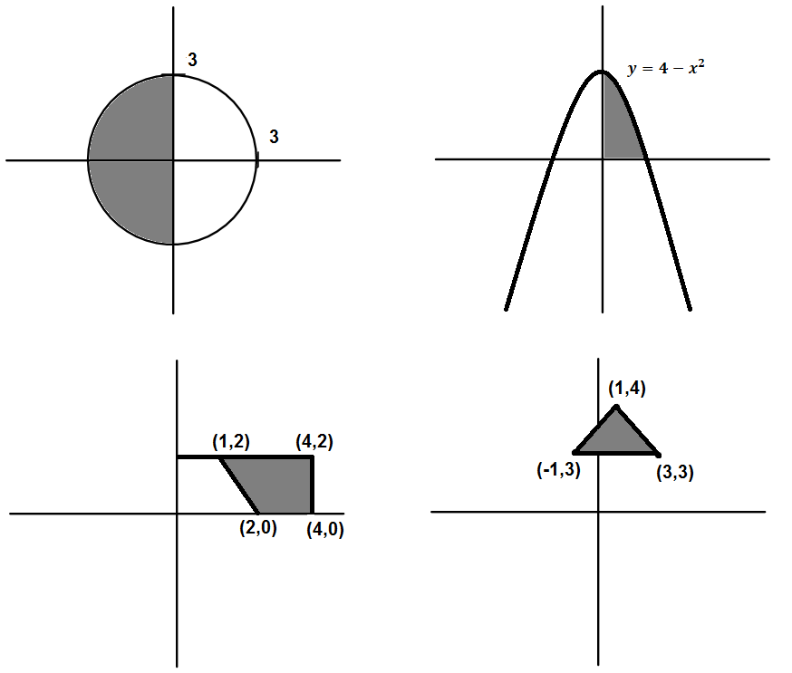
Let \(D\) be the region inside the unit circle centered at the origin, let \(R\) be the right half of \(D\text{,}\) and let \(B\) be the bottom half of \(D\text{.}\)
For each double integral below, decide without calculation whether the double integral will be positive, negative, or zero. You should write a couple of sentences to explain your answer for each part.
The key idea to calculating double integrals using iterated integrals (as shown in Section 12.2 and Preview Activity 12.3.1) is to slice the region of integration along a trace (one of the coordinates held constant) and express the range of the other coordinate in terms of an inequality. In Preview Activity 12.3.1, we saw how the region given in Figure 12.3.2 can be described by the inequalities \(0 \leq x \leq 1\) and \(0 \leq y \leq 1-x\text{.}\) Notice how for different values of \(x\) there is a different range of values for \(y\text{,}\) which means our region is NOT rectangular. Compare this to the rectangular regions of integration from Section 12.2 which were all of the form \(a \leq x \leq b\) and \(c \leq y \leq d\) (with \(a,b,c,d\) constants).
Both of these forms for the inequalities leads to a nice way to write the corresponding double integral as an iterated integral by considering the inner integral to evaluate the cross section area while the outer integral sums up the corresponding cross section volumes as the width of the slices goes to zero (demonstrated in Figure 12.2.4).
What kind of 2D regions can we express using this geometric slicing/inequality idea? The key here is that we need the same upper and lower bound expressions for each slice.
A vertically simple region is one that can be split into vertical slices (of the form \(x=constant\) for \(x\) in the range \([a,b]\)) where every vertical slice has the same upper and lower bound function (\(g_1(x) \leq y \leq g_2(x)\)). A horizontally simple region is one that can be split into horizontal slices (of the form \(y=constant\) for \(y\) in the range \([c,d]\)) where every horizontal slice has the same upper and lower bound functions (\(h_1(x) \leq y \leq h_2(x)\)).
Let \(D\) be the triangular region in the \(xy\)-plane with vertices \((0,0)\text{,}\)\((2,0)\text{,}\) and \((2,3)\text{,}\) shown in Figure 12.3.8. We want to decide if \(D\) is horizontally simple, then we will consider if \(D\) is vertically simple. For simplicity, we will refer to the three sides as the horizontal side (from \((0,0)\) to \((2,0)\)), the vertical side (from \((2,0)\) to \((2,3)\)), and the diagonal side (from \((0,0)\) to \((2,3)\)).
Remember that a vertical line will correspond algebraically to \(x=constant\text{.}\) We want to know if every vertical slice in the region \(D\) will have the same upper and lower bounds (which may depend on the value of \(x\)). Several vertical slices in the region \(D\) are shown in Figure 12.3.9 where you can see that the lower bound (of the \(y\)-variable) for every vertical slice is given by \(y=0\text{.}\) The upper bound (of the \(y\)-variable) for every vertical slice is given by \(y=\frac{3}{2} x\text{.}\) Algebraically, if you take any constant value, \(k\text{,}\) in the interval \([0,2]\text{,}\) then the following statement describes the vertical strips of the region \(D\text{:}\)
\begin{equation*}
\text{Along }x=k\text{ the }y\text{-coordinates go from }0\text{ to }\frac{3}{2}k
\end{equation*}
which corresponds to the inequalities
\begin{equation*}
0\leq x \leq 2 \quad \quad 0 \leq y \leq \frac{3}{2} x
\end{equation*}
as a descriptions for \(D\text{.}\) Thus, the region \(D\) is vertically simple.
Remember that a horizontal line will correspond algebraically to \(y=constant\text{.}\) We want to know if every horizontal slice in the region \(D\) will have the same upper and lower bounds (which may depend on the value of \(y\)). Several horizontal slices in the region \(D\) are shown in Figure 12.3.10 where you can see that the lower bound (of the \(x\)-variable) for every horizontal slice is given by \(x=\frac{2}{3} y\text{.}\) The upper bound (of the \(x\)-variable) for every horizontal slice is given by \(x=2\text{.}\) Algebraically, if you take any constant value, \(k\text{,}\) in the interval \([0,3]\text{,}\) then the following statement describes the horizontal strips of the region \(D\text{:}\)
\begin{equation*}
\text{Along }y=k\text{ the }x\text{-coordinates go from }\frac{2}{3} k\text{ to }2
\end{equation*}
which corresponds to the inequalities
\begin{equation*}
0\leq y \leq 3 \quad \quad \frac{2}{3}y \leq x \leq 2
\end{equation*}
as a descriptions for \(D\text{.}\) Thus, the region \(D\) is horizontally simple.
This example shows that just because a region is vertically simple does not mean that it is not horizontally simple as well. In general, a 2D region is
In this example, we will look at region that is neither horizontally or vertically simple. Let \(D\) be the parallelogram with vertices \((0,0)\text{,}\)\((2,1)\text{,}\)\((4,3)\text{,}\) and \((2,2)\) as shown in Figure 12.3.12. You should take a moment to verify each of the equations for the lines that bound \(D\text{.}\)
If we try to look at \(D\) along vertical slices (of the form \(x=k\)), different values of \(k\) will have different upper and lower bounds. For instance, the default \(k\) value of 0.5 shown in Figure 12.3.13 is a vertical segment with lower bound of \(\left(k,\frac{k}{2}\right)\) and upper bound of \(\left(k,k\right)\text{.}\) You can use the slider at the top of Figure 12.3.13 to change the value of \(k\) to something greater than 2. For values of \(k\) greater than 2, the vertical slice of \(D\) along \(x=k\) will have lower bound of \(\left(k,k-1\right)\) and upper bound of \(\left(k,\frac{k}{2}+1\right)\text{.}\) Because there is not the same upper or lower bounds functions for all vertical slices of \(D\text{,}\)\(D\) is not vertically simple.
If we try to look at \(D\) along horizontal slices (of the form \(y=k\)), different values of \(k\) will have different upper and lower bounds. For instance, the default \(k\) value of 0.5 shown in Figure 12.3.14 is a vertical segment with lower bound of \(\left(k,k\right)\) and upper bound of \(\left(2k,k\right)\text{.}\) You can use the slider at the top of Figure 12.3.14 to change the value of \(k\) to something greater than 1. You can see that for \(k\) values between 1 and 2, the upper bound on the horizontal segment becomes \(\left(k-1,k\right)\) and for \(k\) values above 2, the lower bound will also change to \(\left(\frac{k}{2}+1,k\right)\text{.}\) Because there is not the same upper or lower bounds functions for all vertical slices of \(D\text{,}\)\(D\) is not vertically simple.
In Figure 12.3.15, we have broken our region \(D\) into two regions \(V_1\) and \(V_2\text{.}\) Give inequalities for each of \(V_1\) and \(V_2\) that shows that they are individually vertically simple.
In Figure 12.3.16, we have broken our region \(D\) into three regions \(H_1\text{,}\)\(H_2\text{,}\) and \(H_3\text{.}\) Give inequalities for each of \(H_1\text{,}\)\(H_2\text{,}\) and \(H_3\) that shows that they are individually horizontally simple.
In single variable calculus, we were able to split integrals into multiple parts. The integral of \(f(x)\) over \([a,b]\) could be split to subintervals separately:
Similarly, we can split a region of integration for a double integral into subregions. If a region \(R\) can be split into two sets \(R_1\) and \(R_2\) (where \(R_1\) and \(R_2\) do not overlap), then
\begin{equation*}
\iint_R f(x,y) \, dA = \iint_{R_1} f(x,y) \, dA+\iint_{R_2} f(x,y) \, dA
\end{equation*}
This property is especially useful for a region like Figure 12.3.16 where \(D\) is split into parts \(H_1\text{,}\)\(H_2\text{,}\) and \(H_3\) because
\begin{equation*}
\iint_D f(x,y) \, dA = \iint_{H_1} f(x,y) \, dA+\iint_{H_2} f(x,y) \, dA+\iint_{H_3} f(x,y) \, dA
\end{equation*}
where each of the double integrals on the right can be written as an iterated integral using a horizontally simple description.
For each region, state whether the region is vertically simple, horizontally simple, both, or neither. State the appropriate inequalities to justify when each region is vertically simple or horizontally simple.
Which of the following expressions do not make sense as an iterated integral used to compute a double integral? If the iterated integral does not make sense, explain your reasoning in a couple of sentences. If the iterated integral does make sense, draw a plot of the region of integration.
\begin{equation*}
\int_0^1 \int_1^x f(x,y) \; dy \; dx
\end{equation*}
The process for describing a 2D region as either horizontally or vertically simple is exactly the procedure needed to set up iterated integral that will allow us to evaluate a double integral. If the region \(D\) can be described by the inequalities \(a \leq x \leq b\) and \(g_1(x) \leq y \leq g_2(x)\) (vertically simple), where \(g_1=g_1(x)\) and \(g_2=g_2(x)\) are functions of only \(x\text{,}\) then
\begin{equation*}
\iint_D f(x,y) \, dA = \int_{x=a}^{x=b} \int_{y=g_1(x)}^{y=g_2(x)} f(x,y) \, dy \, dx.
\end{equation*}
Alternatively, if the region \(D\) is described by the inequalities \(c \leq y \leq d\) and \(h_1(y) \leq x \leq h_2(y)\) (horizontally simple), where \(h_1=h_1(y)\) and \(h_2=h_2(y)\) are functions of only \(y\text{,}\) we have
The structure of an iterated integral that will be used to evaluate a double integral should satisfy the following:
the limits on the inner integral must be constants or in terms of outer variable — that is, if the inner integral is with respect to \(y\text{,}\) then its limits may only involve \(x\) and constants, and vice versa.
Let \(f(x,y) = x^2y\) be defined on the triangle \(D\) with vertices \((0,0)\text{,}\)\((2,0)\text{,}\) and \((2,3)\) as shown at left in Figure 12.3.19. This is the same region we described in Activity 12.3.3 and we will use the inequalities from that example to set up our iterated integrals.
To evaluate \(\displaystyle{\iint_D f(x,y) \, dA}\text{,}\) we must first describe the region \(D\) in terms of the variables \(x\) and \(y\text{.}\) We take two approaches corresponding to a vertically simple description, then a horizontally simple description. We will use the inequalities from Activity 12.3.3 that correspond to our vertically simple description:
\begin{equation*}
\text{Along }x=k\text{, the }y\text{-coordinates go from }0\text{ to }\frac{3}{2}k
\end{equation*}
which corresponds to the inequalities
\begin{equation*}
0\leq x \leq 2 \quad \quad 0 \leq y \leq \frac{3}{2} x
\end{equation*}
Using these inequalities corresponds to integrating with respect to \(y\) first (the inner integral).
\begin{equation*}
\iint_D x^2y \, dA = \int_{x=0}^{x=2} \int_{y=0}^{y = \frac32 x} x^2y \, dy \, dx.
\end{equation*}
We evaluate the iterated integral by applying the Fundamental Theorem of Calculus first to the inner integral, and then to the outer one, and find that
We can visualize both the double integral and the iterated integral in Figure 12.3.20. The double integral of \(f(x,y)=x^2y\) over our region \(D\) can be seen as the volume of the region below the surface \(z=f(x,y)\) and above the \(xy\)-plane on the region \(D\text{,}\) shown as the pink volume in Figure 12.3.20.
We can also use each of the iterated integrals to visualize our result. The inner integral corresponds to the area of a cross section along a slice with a fixed \(x\)-value, as shown by the blue cross section in Figure 12.3.20. The result of the inner integral changes depending on which \(x\)-value is used. Algebraically, we see this from our work above that gave \(\frac{9}{8}x^4\) as the result of the inner integral.
To understand this result geometrically, you should use the slider at the top of Figure 12.3.20 to change the \(x\)-value at which the slice of our region is taken and observe that the area of the cross section increases with \(x\text{.}\) The graph of \(\frac{9}{8}x^4\) is projected on a plane and you should notice that as you used the slider to change the \(x\)-value of the slice, the highlighted point on the 2D graph shows the area of slice. The red 2D graph is a plot of the result of the inner integral, which measures the area of cross section at that particular \(x\)-value, which is why the red graph goes higher than the surface \(z\)-values. In fact the peak of the red graph occurs at \(\frac{128}{9}\) where as the highest surface value is \(12\text{.}\) The scale of Figure 12.3.20 has been adjusted to make these features easier to see.
The result of the inner iterated integral is shown by the red graph, so the outer integral will evaluate to be the area under the red graph, which is shown in orange on the 2D graph portion of Figure 12.3.20. Again, remember that the outer integral evaluates the Riemann sum corresponding to the cross sectional volumes (like in Figure 12.2.4).
In the previous task, we use a vertically simple description for the region of integration \(D\text{,}\) which allowed use an iterated integral where we integrated with respect to \(y\) first (while treating \(x\) as a constant) and then integrating across the interval of relevent \(x\)-values. In this task, we will use a horizontally simple description for our region of integration and as a consequence the order in which we integrate our variables will be switched.
Similar to our visualization description for the vertically simple case, we can look at our double integral from a different perspective to understand the different parts of our iterated integral. In Figure 12.3.21, you can see the same volume as before in pink which corresponds to the volume computed by the double integral. In this task, we used a horizontally simple description which means our slices correspond to constant values of \(y\text{.}\) The cross sectional area of this slice along a constant \(y\)-value is shown in blue on both the slice of our volume and on the 2D graph that shows the values of the inner integral (as a function of \(y\)). You can use the slider at the top of Figure 12.3.21 to see how the area of cross section changes with respect to different values of \(y\text{.}\)
You can see that as \(y\) increases from 0, the value of cross sectional area increases for a while, then decreases. While the height of our surface is increasing with respect to \(y\) over \([0,3]\text{,}\) the length of the slice is getting smaller as \(y\) increases. This is captured algebraically by our inner integral in that the function we are integrating (\(x^2y\)) is increasing but the length of the interval we are integrating over (\(\frac{2}{3}y\leq x\leq2\)) is decreasing as we increase \(y\text{.}\) This is why our 2D graph in ends up having a concave down shape.
Again, we can visualize the cross section areas as the height of red graph, which will allow us to consider the value the double integral to be the area under the red curve (in our 2D plot). While the orange area in Figure 12.3.21 may look less than the orange area in Figure 12.3.20, they are in fact the same. The width of the orange area in Figure 12.3.21 is 3, whereas the width of the orange area in Figure 12.3.20 is two.
We see that in the situation where \(D\) can be described as horizontally simple or vertically simple, the order in which we choose to set up and evaluate the iterated integrals doesn’t matter; the same value results in either case.
The process of switching between a vertically simple description and a horizontally simple description for the region of integration is often called switching the order of integation because the corresponding iterated integrals used to calculate a double integral will have the order in which you integrate these variables switched.
The meaning of a double integral over a non-rectangular region, \(D\text{,}\) parallels the meaning over a rectangular region. In particular,
\(\displaystyle{\iint_D f(x,y) \, dA}\) tells us the volume of the solids the graph of \(f\) bounds above the \(xy\)-plane over the closed, bounded region \(D\) minus the volume of the solids the graph of \(f\) bounds below the \(xy\)-plane under the region \(D\text{;}\)
\(\displaystyle{\frac{1}{A(D)} \iint_R f(x,y) \, dA}\text{,}\) where \(A(D)\) is the area of \(D\) tells us the average value of the function \(f\) on \(D\text{.}\) If \(f(x, y) \geq 0\) on \(D\text{,}\) we can interpret this average value of \(f\) on \(D\) as the height of the solid with base \(D\) and constant cross-sectional area \(D\) that has the same volume as the volume of the surface defined by \(f\) over \(D\text{.}\)
If \(f(x,y)\) measure the density (in amount per unit area) of a material in the region \(D\text{,}\) then \(\iint_D f(x,y) \, dA\) will give the total amount of material in \(D\text{.}\)
In the next activity, we will practice the process of understanding a region of integration, using horizontally simple and vertically simple descriptions of the region, setting up and evaluating the corresponding iterated integrals.
Consider the double integral \(\displaystyle{\iint_D (4-x-2y) \, dA}\text{,}\) where \(D\) is the triangular region with vertices (0,0), (4,0), and (0,2).
Draw and label a plot of \(D\) with relevent cross sections for a vertically simple description. Give the inequalities that show \(D\) as vertically simple.
Draw and label a plot of \(D\) with relevent cross sections for a horizontally simple description. Give the inequalities that show \(D\) as horizontally simple.
Evaluate the two iterated integrals from the previous two parts, and verify that they produce the same value. Give at least one interpretation of the meaning of your result.
In the next activity, we will explore to understand a region of integration, with some non-linear sides, given as bounds in an iterated integral, then we will switch the order of integration, evaluate which ever order is most convinient and finally interpret the result using the average value approach.
Determine the equivalent iterated integral that results from integrating in the opposite order (\(dx \, dy\text{,}\) instead of \(dy \, dx\)). That is, determine the limits of integration for which
In the following activity, we will explore how switching the order of integration can sometimes yield a much easier set of iterated integral to evaluate algebraically.
Explain why we cannot find a simple antiderivative for \(e^{y^2}\) with respect to \(y\text{,}\) and thus are unable to evaluate \(\int_{x=0}^{x=4} \int_{y=x/2}^{y=2} e^{y^2} \, dy \, dx\) in the indicated order using the Fundamental Theorem of Calculus.
Use the Fundamental Theorem of Calculus to evaluate the iterated integral you developed in (c). Write one sentence to explain the meaning of the value you found.
For a double integral \(\displaystyle{\iint_D f(x,y) \, dA}\text{,}\) we can write appropriate iterated integrals if the region \(D\) is either horizontally or vertically simple. A horizontally simple region is described by the inequalities \(c \leq y \leq d\) and \(h_1(y) \leq x \leq h_2(y)\) . A vertically simple region is described by \(a \leq x \leq b\) and \(g_1(x) \leq y \leq g_2(x)\text{.}\)
In an iterated double integral, the limits on the outer integral must be constants while the limits on the inner integral must be constants or in terms of only the remaining variable. In other words, an iterated integral corresponding to a double integral has one of the following forms (which result in the same value):
\begin{equation*}
\int_{x=a}^{x=b} \int_{y=g_1(x)}^{y=g_2(x)} f(x,y) \, dy \, dx,
\end{equation*}
where \(g_1=g_1(x)\) and \(g_2=g_2(x)\) are functions of \(x\) only and the region \(D\) is described by the inequalities \(a \leq x \leq b\) and \(g_1(x) \leq y \leq g_2(x)\) or
where \(h_1=h_1(y)\) and \(h_2=h_2(y)\) are functions of \(y\) only and the region \(D\) is described by the inequalities \(c \leq y \leq d\) and \(h_1(y) \leq x \leq h_2(y)\text{.}\)
Evaluate the double integral \(\displaystyle I = \int\!\!\int_{\mathbf{D}} xy \: d\!A\) where \(\mathbf{D}\) is the triangular region with vertices \((0, 0), (6, 0), (0, 1)\text{.}\)
Evaluate the double integral \(\displaystyle I = \int\!\!\int_{\mathbf{D}} xy \: d\!A\) where \(\mathbf{D}\) is the triangular region with vertices \((0, 0), (1, 0), (0, 5)\text{.}\)
Decide, without calculation, if each of the integrals below are positive, negative, or zero. Let D be the region inside the unit circle centered at the origin. Let T, B, R, and L denote the regions enclosed by the top half, the bottom half, the right half, and the left half of unit circle, respectively.
(a) Think about what the contours of \(f\) look like. You may want to using \(f(x,y)=1\) as an example. Sketch a rough contour diagram on a separate sheet of paper.
(c) Use your work from (b) to write an iterated double integral giving the volume of \(W\text{,}\) using the work from (b) to inform the construction of the inside integral.
Set up a double integral in rectangular coordinates for calculating the volume of the solid under the graph of the function \(f(x,y) = 22-x^{2}-y^{2}\) and above the plane \(z = 6\text{.}\)
Instructions: Please enter the integrand in the first answer box. Depending on the order of integration you choose, enter dx and dy in either order into the second and third answer boxes with only one dx or dy in each box. Then, enter the limits of integration.
Consider the integral \(\displaystyle \int_0^6 \int_0^{\sqrt{36-y}} f(x,y) dx dy\text{.}\) If we change the order of integration we obtain the sum of two integrals:
A pile of earth standing on flat ground has height 36 meters. The ground is the xy-plane. The origin is directly below the top of the pile and the z-axis is upward. The cross-section at height z is given by \(x^2 + y^2 = 36 - z\) for \(0 \leq z \leq 36\text{,}\) with \(x, y,\) and \(z\) in meters.
Match the following integrals with the verbal descriptions of the solids whose volumes they give. Put the letter of the verbal description to the left of the corresponding integral.
The temperature at any point on a metal plate in the \(xy\)-plane is given by \(T(x,y) = 100-4x^2 - y^2\text{,}\) where \(x\) and \(y\) are measured in inches and \(T\) in degrees Celsius. Consider the portion of the plate that lies on the region \(D\) that is the finite region that lies between the parabolas \(x = y^2\) and \(x = 3 - 2y^2\text{.}\)
Construct a labeled sketch of the region \(D\text{.}\)
Set up an iterated integral whose value is \(\iint_D T(x,y) \, dA\text{,}\) using \(dA = dx dy\text{.}\) (Hint: It is possible that more than one integral is needed.)
Set up an integrated integral whose value is \(\iint_D T(x,y) \, dA\text{,}\) using \(dA = dy dx\text{.}\) (Hint: It is possible that more than one integral is needed.)
Consider the solid that is given by the following description: the base is the given region \(D\text{,}\) while the top is given by the surface \(z = p(x,y)\text{.}\) In each setting below, set up, but do not evaluate, an iterated integral whose value is the exact volume of the solid. Include a labeled sketch of \(D\) in each case.
\(D\) is the interior of the quarter circle of radius 2, centered at the origin, that lies in the second quadrant of the plane; \(p(x,y) = 16-x^2-y^2\text{.}\)