In this preview activity, we will investigate some measurements that will be useful when defining new ways to specify locations. Many of these measurements involve measuring the length of specific line segments and angles between line segments in three dimensions.
An angle in the \(xy\)-plane is in standard position if the initial side of the angle is on the positive \(x\)-axis and is measured with the positive direction going counterclockwise.
If an angle \(\theta\) is in standard position, for which quadrants will \(\sin(\theta)\) be positive? For which quadrants will \(\sin(\theta)\) be negative? Which angles correspond to \(\sin(\theta)=0\text{?}\)
If an angle \(\theta\) is in standard position, for which quadrants will \(\cos(\theta)\) be positive? For which quadrants will \(\cos(\theta)\) be negative? Which angles correspond to \(\cos(\theta)=0\text{?}\)
If an angle \(\theta\) is in standard position, for which quadrants will \(\tan(\theta)\) be positive? For which quadrants will \(\tan(\theta)\) be negative? Which angles correspond to \(\tan(\theta)=0\text{?}\) Which angles correspond to \(\tan(\theta)\) being undefined?
A three dimensional plot with the point \(P\) labeled and drawn with a green segment parallel to the z-axis. The green segment is labeled 2. A red segment is drawn perpendicular to the x-axis to the end point of the green segment on the xy-plane. The red segment is labeled 3. A blue segment goes from the origin to the point at which the green segment hits the xy-plane and is labeled 5.
The angle in the \(xy\)-plane between the \(x\)-axis and the line segment (in blue) labeled \(5\) that is from the origin to a point directly below \(P\text{.}\)
A three dimensional plot with the point labeled \(P\) is below the xy-plane and drawn with a green segment parallel to the z-axis. The green segment is labeled 1. A red segment is drawn perpendicular to the negative x-axis to the end point of the green segment on the xy-plane. The red segment is labeled 2. A blue segment goes from the origin to the point at which the green segment hits the xy-plane and is labeled 3. A pink segment from the origin is drawn to the point \(P\text{.}\) An orange arc is drawn in the same plane as the blue and pink segments and extends down from the positive z-axis to the pink segment.
In this section we will define and work with new ways to specify the location of a point. These new measurements will be useful as coordinate systems and as a way of thinking about how to describe different shapes relative to rotational or other symmetries.
We previously defined the rectangular coordinates of a point to be signed distances from the point to the axes as shown below. Remember that the sign on the coordinate tells you whether to go above or below the other axis.
We define the polar coordinates of a point \(P\) in two dimensions to be \((r,\theta)\text{,}\) where \(r\) is the signed distance from the origin to \(P\) and \(\theta\) is the counterclockwise angle from the positive horizontal axis to the line segment connecting the origin and \(P\text{.}\) We use the sign on the \(r\) to indicate if the point is locked ahead or behind when facing the \(\theta\) direction at the origin.
A two dimensional plot with the horizontal axis labeled \(x\text{,}\) the vertical axis labeled \(y\text{,}\) and a point labeled \(P=(r,\theta)\text{.}\) Additionally, there is a red segment going from the origin up and to the right, with end point at \(P\text{.}\) The red segment is labeled \(r\text{.}\) A blue arc is shown going counterclockwise from the horizontal axis to the red segment and is labeled \(\theta\text{.}\)
A helpful way to visualize a location based on polar coordinates is to stand at the origin, facing the positive horizontal axis; turn an angle of \(\theta\) counterclockwise; and move \(r\) in the direction you are facing.
Our first example will look at the location given by \(P:(r,\theta)=(2,\frac{\pi}{2})\text{.}\) To understand where this point is, we do the following steps: from the origin, face the positive \(x\)-axis; turn \(\frac{\pi}{2}\) radians counterclockwise (to the positive \(y\) axis); and move two units in the direction you are now facing.
A two dimensional plot with the horizontal axis labeled x, the vertical axes labeled y, and an arrow pointing from the origin to the right, labeled "Face this way".
A two dimensional plot with the horizontal axis labeled x, the vertical axes labeled y, and an arrow pointing up from the origin, labeled "Face this way". A blue circular arc is drawn with arrow counterclockwise from the positive horizontal axis to the positive vertical axis.
A two dimensional plot with the horizontal axis labeled x, the vertical axes labeled y, and an arrow pointing up from the origin, labeled "Face this way". A blue circular arc is drawn with arrow counterclockwise from the positive horizontal axis to the positive vertical axis. A red segment is drawn vertically from the origin to a point labeled \(P:(r,\theta)=(2,\pi//2)\text{.}\)
Geometrically, we can see that this location would have rectangular coordinates of \((x,y)=(0,2)\text{.}\) While geometry is useful for understanding meaning, it is rarely wise to compute things like coordinates using only a graph. Later in this section, we will talk about algebraic tools that will allow us to convert between rectangular and polar coordinates.
A two dimensional plot with the horizontal axis labeled x, the vertical axes labeled y, and an arrow pointing from the origin to the right, labeled "Face this way".
A two dimensional plot with the horizontal axis labeled x, the vertical axes labeled y, and an arrow pointing down from the origin, labeled "Face this way". A blue circular arc is drawn with arrow clockwise from the positive horizontal axis to the negative vertical axis.
A two dimensional plot with the horizontal axis labeled x, the vertical axes labeled y, and an arrow pointing down from the origin, labeled "Face this way". A blue circular arc is drawn with arrow clockwise from the positive horizontal axis to the negative vertical axis. The blue arc is labeled \(\theta=-\frac{\pi}{4}\text{.}\) A red segment is drawn vertically up from the origin to a point labeled \(Q:(r,\theta)=(-2,-\pi//2)\text{.}\)
Notice that both \(P:(r,\theta)=(2,\frac{\pi}{2})\) and \(Q:(r,\theta)=(-2,-\frac{\pi}{2})\) correspond to the location with rectangular coordinates \((0,2)\text{.}\) This example highlights how polar coordinates are measured and how there is not a unique set of polar coordinates for a location.
If you look at Figure 9.8.4, you can see a right triangle in the first quadrant with base \(x\) and height \(y\text{.}\) The angle the hypotenuse makes with the base is \(\theta\text{.}\) From this, you can deduce the four relationships shown below, which are used to convert between rectangular and polar coordinates. It may be insightful to draw triangles of this type in each of the quadrants to confirm for yourself that these conversion formulas are valid in all four cases.
It is important to notice that the equations used in the conversion from polar to rectangular work to convert coordinates of a point for any values of \(r\) and \(\theta\text{,}\) including negative \(r\)-values and values of \(\theta\) outside the interval \([0,2\pi]\text{.}\) The conversion equations to go from rectangular to polar require you to interpret the results of your calculation by choosing from multiple suitable values for \(r\) and \(\theta\text{.}\) This is because we are not able to solve uniquely for \(r\) and \(\theta\) in terms of \(x\) and \(y\text{.}\) This is because there is not a unique set of polar coordinates for a location. A point can have many different polar coordinates that refer to the same location.
For example, the point with rectangular coordinates \((-1,-1)\) can be given the polar coordinates \((r,\theta)=(\sqrt{2},\frac{5\pi}{4})\) or \((r,\theta)=(-\sqrt{2},\frac{-\pi}{4})\) or \((r,\theta)=(\sqrt{2},\frac{13\pi}{4})\) or \((r,\theta)=(\sqrt{2},-\frac{3\pi}{4})\) or \((r,\theta)=(-\sqrt{2},-\frac{7\pi}{4})\) (amongst many others). The good news is that when you need to choose appropriate \(r\) and \(\theta\text{,}\) you can make proper choices based on your experience with quadrants and where the point is (in terms of \(x\) and \(y\)).
In this example, we will look at how to convert the points with rectangular coordinates \(P=(-2,3)\) and \(Q=(-3,-2)\) into polar coordinates. Note here that \(P\) is in the second quadrant and \(Q\) is in the third quadrant.
which means we need to pick \(r\) to be \(\sqrt{13}\) or \(-\sqrt{13}\text{.}\) We will need to pick a appropriate angles for these possible \(r\)-values that satisfy \(\tan(\theta) = -\frac{3}{2}\text{.}\) There are angles in the fourth and second quadrants that will satisfy \(\tan(\theta) = -\frac{3}{2}\text{,}\) namely \(\arctan(-\frac{3}{2})\) and \(\pi +\arctan(-\frac{3}{2})\text{.}\) You could also choose any angle coterminal to either of these angles. This is not a situation where we can arbitrarily combine one of the choices of \(r\) will work with any choice of \(\theta\text{.}\) We must interpret these choices together to get a description for the correct location.
If we choose \(r=\sqrt{13}\text{,}\) then we need to select the angle that corresponds to the second quadrant, \(\pi + \arctan(-\frac{3}{2})\text{,}\) to get polar coordinates \(P=(r,\theta)=(\sqrt{13},\pi+\arctan(-\frac{3}{2}))\text{.}\) If we want to not have to use the complementary angle to \(\arctan(-\frac{3}{2})\text{,}\) then we need to use the negative value of \(r\) to get \(P=(r,\theta)=(-\sqrt{13},\arctan(-\frac{3}{2}))\text{.}\)Figure 9.8.13 illustrates these two different polar coordinates that identify the point \(P\)
A two dimensional plot with coordinates going from negative four to four. A point is shown two to the right and three up from the origin and labeled \(P\text{.}\) A red segment is drawn from the origin to the point \(P\text{.}\) A blue dashed line is drawn from the origin in the opposite direction of the red segment. A blue circular arc is drawn clockwise from the positive horizontal axis to the blue dashed line and is labeled \(\arctan(-\frac{3}{2})\text{.}\)
A two dimensional plot with coordinates going from negative four to four. A point is shown two to the right and three up from the origin and labeled \(P\text{.}\) A red segment is drawn from the origin to the point \(P\text{.}\) A blue dashed line is drawn from the origin in the opposite direction of the red segment. A blue circular arc is drawn clockwise from the positive horizontal axis to the blue dashed line and is labeled \(\arctan(-\frac{3}{2})\text{.}\) A green circular arc is drawn counterclockwise from the positive horizontal axes to the red segment and is labeled \(\pi+\arctan(-\frac{3}{2})\text{.}\)
Now we will look at how to convert \(Q=(-3,-2)\) into polar coordinates. Similar to our arguments above, we find that \(Q=(-3,-2)\) implies that \(r^2=9+4=13\) and \(\tan(\theta)=\frac{-2}{-3}\text{.}\) If we want to consider a positive value for \(r\) and a value of \(\theta\) between \(0\) and \(2\pi\text{,}\) then we get \(r=\sqrt{13}\) and \(\theta=\pi+\arctan(\frac{2}{3}) \text{.}\) We could also consider a negative value for \(r\) and a value of \(\theta\) between \(0\) and \(2\pi\text{,}\) which would yield \(r=-\sqrt{13}\) and \(\theta=\arctan(\frac{2}{3}) \text{.}\)Figure 9.8.14 illustrates these two perspectives on finding polar coordinates for \(Q\)
A two dimensional plot with coordinates going from negative four to four. A point is shown three to the right and two down from the origin and labeled \(Q\text{.}\) A red segment is drawn from the origin to the point \(Q\) and is labeled \(\sqrt{13}\text{.}\) A blue dashed line is drawn from the origin in the opposite direction of the red segment. A blue circular arc is drawn counterclockwise from the positive horizontal axis to the green dashed line and is labeled \(\arctan(\frac{2}{3})\text{.}\) A green circular arc is drawn counterclockwise from the positive horizontal axes to the red segment and is labeled \(\pi+\arctan(\frac{2}{3})\text{.}\)
A two dimensional plot with coordinates going from negative four to four. A point is shown three to the right and two down from the origin and labeled \(Q\text{.}\) A red segment is drawn from the origin to the point \(Q\) and is labeled \(-\sqrt{13}\text{.}\) A blue dashed line is drawn from the origin in the opposite direction of the red segment. A blue circular arc is drawn counterclockwise from the positive horizontal axes to the dashed blue line and is labeled \(\arctan(\frac{2}{3})\text{.}\)
Remember that inverse trig functions have limited domains and ranges, the \(r\)-coordinate can be positive or negative, and polar coordinates do not have unique values for a given point.
Compute the exact value of \(r\) and \(\theta\) for each point. Exact values include things like \(\sqrt{3}\text{,}\)\(\arcsin(3/4)\text{,}\) etc. Simplify trigonometric function values of any common angles you encounter, like \(\sin\left(\frac{\pi}{3}\right)=\frac{\sqrt{3}}{2}\text{.}\)
Compute the exact value of \(x\) and \(y\) for each point. Exact values include things like \(\sqrt{3}\text{,}\)\(\arcsin(3/4)\text{,}\) etc. Simplify trigonometric function values of any common angles you encounter, like \(\sin\left(\frac{\pi}{3}\right)=\frac{\sqrt{3}}{2}\text{.}\)
We now want to look at converting an equation between rectangular and polar coordinates. Remember that the graph of an equation is the set of all points that satisfy the equation. When we say that we want to convert an equation such as \(x=y^2\) to polar coordinates, we mean that we want to find an equation in \(r\) and \(\theta\) whose graph will be exactly the same set of points as \(x=y^2\text{.}\) This will be fairly easy because we have conversion equations that are solved explicitly and uniquely for \(x\) and \(y \text{:}\)\(x=r\cos(\theta)\) and \(y=r\sin(\theta)\text{.}\)
We can convert the equation \(x=y^2\) to polar coordinates by substituting \(x=r\cos(\theta)\) and \(y=r\sin(\theta)\) to get
\begin{align*}
x \amp= y^2 \\
r \cos(\theta) \amp= (r \sin(\theta))^2 \\
r \cos(\theta) \amp= r^2 \sin(\theta)^2 \\
\frac{\cos(\theta)}{\sin(\theta)^2} \amp= r\\
r \amp= \cot(\theta) \csc(\theta)
\end{align*}
This tells us that the \((r,\theta)\) points satisfying \(r = \cot(\theta) \csc(\theta)\) are the same locations as the \((x,y)\) points that satisfy \(x=y^2\text{.}\)Except, we divided by \(\sin(\theta)\text{,}\) which will not give an equivalent equation if \(\sin(\theta)=0\text{.}\) Notice that if \(\theta=0\) (or any integer multiple of \(\pi\)), then \(\cot(\theta) \csc(\theta)\) does not exist. In a technical sense, we would either need to stop our algebra at \(\cos(\theta)=r \sin(\theta)^2\) or use a piecewise defined expression such as
\begin{equation*}
r= \begin{cases}
0 \amp \theta=k\pi \text{ for } k \in \mathbb{Z} \\
\cot(\theta) \csc(\theta) \amp \theta \neq k\pi \text{ for } k \in \mathbb{Z}
\end{cases}
\end{equation*}
This example highlights the tricky part of converting equations: without careful algebraic steps, you can miss points that need to be included in the graphs/equations or possibly get nonsensical statements. Often we will use geometric intuition and information to help convert equations between coordinate systems and make sense of the resulting expressions.
The previous example showed that converting an equation from rectangular coordinates to polar coordinates is mostly straightforward, although we must pay attention to issues where expressions may become undefined. Our next example focuses on the conversion from polar to rectangular coordinates, which has additional subtleties.
In this example, we will convert the equation \(r=3\cos(\theta)\) into rectangular coordinates, identify the shape of its graph, and plot its graph. Remember that we do not have conversion equations for \(r\) and \(\theta\text{,}\) but we do have some equations relating the variables, such as \(r^2=x^2+y^2\text{.}\) This will allow us to convert to an expression in \(x\) and \(y\) that does not require interpretation. We start by squaring both sides of our polar equation, since this will give us an expression on the left-hand side of the equation that will be easy to convert to rectangular coordinates. This yields
Our last equation is a mix of rectangular and polar coordinates so we are not done with our conversion to rectangular coordinates. Unfortunately the easiest way to convert \((\cos(\theta))^2\) to rectangular is to use
which will give us a rational expression for our conversion. This would require some extra algebra and interpretation, so let’s try a slightly different approach.
Instead of squaring both sides of our polar equation, we can start by multiplying both sides by \(r\text{.}\) You may have seen this as a better approach from the start or gained this insight after our work above.
After we multiply both sides of our original equation by \(r\text{,}\) we have
\begin{equation*}
r =3\cos(\theta) \Rightarrow r^2=3 r \cos(\theta)
\end{equation*}
This equation is great because both the left and right hand sides have explicit conversions to rectangular coordinates that do not require separate interpretation of quadrants. Thus, we see that the \((r,\theta)\) points that satisfy \(r = 3 \cos(\theta)\) are the same locations as the \((x,y)\) points that satisfy \(x^2+y^2=3x\text{.}\)
We have now converted our polar equation to a rectangular equation. What shape will the graph of \(x^2+y^2=3x\) (or \(r = 3 \cos(\theta)\)) be? We can use the algebraic technique of completing the square to transform our equation into the the standard form of a circle: \((x-h)^2+(y-k)^2 = R^2\text{.}\)
We can see now that this circle will have center \((\frac{3}{2},0)\) and radius \(\frac{3}{2}\text{.}\) The graph of \(r =3\cos(\theta)\) is the same as \(x^2+y^2=3x\) or \((x -\frac{3}{2})^2 +(y-0)^2 =\left(\frac{3}{2}\right)^2\text{,}\) which is plotted below.
While many people will find the rectangular equation more comfortable to graph and work with, this conversion from polar to rectangular is not always needed. You can find many resources on plotting points of a polar equation without converting to rectangular coordinates, especially when one coordinate (typically \(r\)) is solved explicitly in terms of the other coordinate.
A plot of a circle with center 1.5 units to the right of the origin and with radius 1.5 units. A blue segment is drawn from the origin to a point that is 1.5 units to the right and 1.5 units down. This end point of the blue segment is labeled \(P:(r,\theta)=(\sqrt{3},-\arctan(\frac{\sqrt{2}}{2}))\text{.}\) A blue circular arc is drawn clockwise from the positive horizontal axis to the blue segment and is labeled \(-\arctan(\frac{\sqrt{2}}{2})\text{.}\)
Consider the polar equation \(r=\cos(\theta)\text{.}\) Complete the table below by computing the value of \(r\) for each value of \(\theta\) for this equation.
Plot each of the eleven points you found in the previous part on the polar plane and connect them to make a plot of the graph of \(r=\cos(\theta)\text{.}\)
Now that you have some experience with plotting polar equations, the next activity will allow you to practice converting between polar and rectangular forms and seeing how graphs can help you with understanding these equations.
You may find it useful to have an intermediate step with an equation involving both \(r\) and \(x\) and completing the square as in Example 9.8.16 will likely be useful as well.
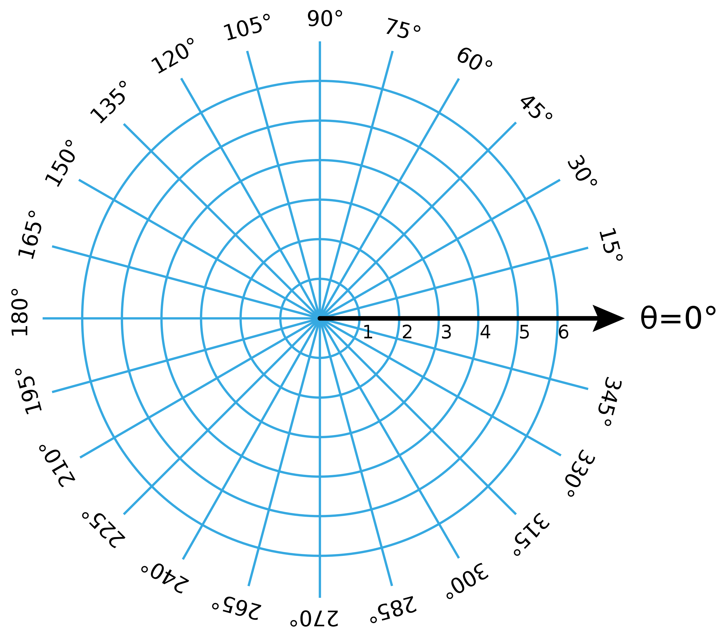
In Figure 9.1.1, you saw how a rectangular grid makes it easy to determine the rectangular coordinates of a point. A polar grid gives the same tools by plotting an array of constant coordinate graphs. An example of a polar grid is given in Figure 9.8.19, and thinking about this polar grid should help you answer the questions in Activity 9.8.5
A plot consisting of six concentric circles centered at the origin as well as rays emanating from the origin in \(15^\circ\) increments from \(0^\circ\) to \(345^\circ\text{.}\)
Write a couple of sentences describing the graph of \(r=c\text{,}\) where \(c\) is a constant. You should consider what values of \(c\) will correspond to different shapes.
Write a couple of sentences describing the graph of \(\theta=d\text{,}\) where \(d\) is a constant. You should consider what values of \(d\) will correspond to different shapes.
The last idea of conversion we will look at between rectangular and polar coordinates is how to convert regions or inequalities between coordinate systems. Just as a graph of a an equation is a plot of the set of points that satisfies the equation, the graph of an inequality (or set of inequalities) is the region of points that satisfy the inequality.
The graph of the inequality \(-1\leq x \leq 1\) is the vertical strip of points with horizontal coordinate between \(-1\) and \(1\) (inclusive) and has graph shown in Figure 9.8.21.
A two dimensional plot with coordinates going from negative three to three. A rectangular region that extends one unit right and left of the vertical axis is highlighted in green. The vertical lines that are the boundary of this region are drawn with black lines.
If we consider the set of inequalities given by \(-1\leq x \leq 1\) and \(0\leq y \leq 2\text{,}\) then we are looking for the region of points that satisfies both inequalities. The second inequality is shown in red in Figure 9.8.22.(a) and the intersection of the two plots corresponds to the region described by \(-1\leq x \leq 1\) and \(0\leq y \leq 2\text{,}\) which is plotted in blue Figure 9.8.22.(b).
A two dimensional plot with coordinates going from negative three to three. A rectangular region that extends from the horizontal axis to two units above the horizontal axis is highlighted in red. The horizontal lines that are the boundary of this region are drawn with black lines.
A two dimensional plot with coordinates going from negative three to three. A square region that goes one unit to the right and left of the vertical axis and from the horizontal axis to two units above the horizontal axis is shown in blue. The rest of the rectangular region that extends one unit right and left of the vertical axis is highlighted in green. The vertical lines that are the boundary of this region are drawn with black lines. The rest of the rectangular region that extends one unit right and left of the vertical axis is highlighted in green. The vertical lines that are the boundary of this region are drawn with black lines.
Plot the region that corresponds to the polar inequality \(\frac{\pi}{4} \leq \theta \leq \frac{3\pi}{4}\text{.}\) Write a sentence or two to describe this region.
Plot the region that corresponds to the polar inequalities \(1 \leq r \leq 3\) and \(\frac{\pi}{4} \leq \theta \leq \frac{3\pi}{4}\text{.}\) Write a sentence or two to describe this region.
So far in this chapter, we have encountered two different coordinate systems in \(\R^2\text{:}\) rectangular and polar coordinates. Earlier in this section, we saw how polar coordinates form a convenient alternative in certain situations. In a similar way, there are two more coordinate systems in \(\R^3\) that come from different ideas of rotational measurement. This subsection introduces cylindrical coordinates, which we can view as a vertical extension of polar coordinates to three dimensions. The next subsection will introduce spherical coordinates, which are useful for situations with significant rotational symmetry with respect to the origin.
Cylindrical coordinates are a coordinate system for \(\mathbb{R}^3\) that consists of using polar coordinates, \(r\) and \(\theta\text{,}\) in place of \(x\) and \(y\) coordinates. Cylindrical coordinates are given in the order of \((r,\theta,z)\) and can be described as “polar plus \(z\)”. The \(z\)-coordinate is measured the same way as in rectangular coordinates (signed distance above or below the \(xy\)-plane) and polar coordinates are measured as a projection of the point in three dimensions onto the \(xy\)-plane. To convert between rectangular and cylindrical coordinates, we use the same conversion equations as between rectangular and polar coordinates (in two dimensions).
A three dimensional plot is shown with the xy-plane highlighted with a gridded gray plane. A point in the positive x,y,z directions is drawn and labeled \(P=(r,\theta,z)\text{.}\) A green segment is drawn parallel to the z-axis, from the point \(P\) to the xy-plane and is labeled \(z\text{.}\) A red segment is drawn from axis labeled \(x\) to the point where the green segment intersects the xy-plane and is labeled \(r\text{.}\) A blue circular arc is drawn in the xy-plane from the axis labeled \(x\) to the red segment.
For our first example, we will look at the point with cylindrical coordinates \((r,\theta,z)=\left(\sqrt{5},\frac{3\pi}{4},-2\right)\text{.}\) This point is shown in Figure 9.8.25 with the measurements of the cylindrical coordinates.
A three dimensional plot is shown with the xy-plane highlighted with a gridded gray plane. A point in direction of the axis labeled \(y\) and opposite direction of the axes labeled \(x\) and \(z\text{.}\) A green segment is drawn parallel to the z-axis, from the point up to the xy-plane and is labeled \(-2\text{.}\) A red segment is drawn from axis labeled \(x\) to the point where the green segment intersects the xy-plane and is labeled \(r\text{.}\) A blue circular arc is drawn in the xy-plane from the axis labeled \(x\) to the red segment. The blue arc is labeled \(\theta\text{.}\)
To convert our cylindrical coordinates to rectangular, we can use \(x = r \cos(\theta)\) and \(y = r \sin(\theta)\text{.}\) This gives rectangular coordinates of \((x,y,z)= \left(-\frac{\sqrt{10}}{2},\frac{\sqrt{10}}{2},-2\right)\text{.}\)
Next, we will find cylindrical coordinates for the point with rectangular coordinates \((x,y,z)=(-2,1,2)\text{.}\) Just as the polar coordinates of a point in two dimensions are not unique, the cylindrical coordinates of a point in three dimensions will not be unique.
Using our conversion equations from rectangular to cylindrical, we get \(r^2=(-2)^2+(1)^2=5\) and \(\tan(\theta)= \frac{1}{-2}\text{.}\) Remember that we must interpret the angle and our choice of \(r\) to make sure our coordinates describe a point in the second octant. In particular, we will choose a positive \(r\) value of \(\sqrt{5}\) which means we will need to select \(\theta = \arctan\left(-\frac{1}{2}\right)+\pi\text{.}\)
Alternatively, we can use \(\cos(\theta)=\frac{x}{r}\) since \(\arccos\) will give an output of an angle in the first or second quadrants. You can verify that \(\theta = \arctan\left(-\frac{1}{2}\right)+\pi = \arccos\left(-\frac{2}{\sqrt{5}}\right)\text{.}\) So rectangular coordinates \((x,y,z)=(-2,1,2)\) will correspond to cylindrical coordinates of \((r,\theta,z)= \left(\sqrt{5},\arctan\left(-\frac{1}{2}\right)+\pi,2\right)\) or \((r,\theta,z)= \left(\sqrt{5},\arccos\left(-\frac{2}{\sqrt{5}}\right),2\right) \text{.}\)
A three dimensional plot is shown with the xy-plane highlighted with a gridded gray plane. A point in direction of the axes labeled \(y\) and \(z\) and opposite direction of the axis labeled \(x\text{.}\) A green segment is drawn parallel to the z-axis, from the point down to the xy-plane and is labeled \(2\text{.}\) A red segment is drawn from axis labeled \(x\) to the point where the green segment intersects the xy-plane and is labeled \(r\text{.}\) A blue circular arc is drawn in the xy-plane from the axis labeled \(x\) to the red segment. The blue arc is labeled \(\theta\text{.}\) A pink segment is drawn two units from the origin in the direction opposite the axis labeled \(x\text{.}\) From the end of the pink segment, there is a dark red segment of length one unit drawn parallel to the axis labeled \(y\text{.}\)
When introducing polar coordinates, we saw how the graph of \(\theta=2\) is a line with slope \(\tan(2)\text{.}\) If we consider only positive \(r\) coordinates then we get a ray with an angle of \(2\) radians from the positive \(x\)-axis. If we wanted to consider the graph in three dimensions of \(\theta=2\) using cylindrical coordinates, then we have a plane containing the \(z\)-axis and extending in the \(\theta=2\) direction. This is a cylinder surface with the line given by \(y=\tan(2) x\) as the generating curve and rulings parallel to the \(x\)-axis.
A three dimensional plot with a half plane extending from the axis labeled \(z\) in the direction of positive \(y\) and negative \(x\) axes shown in blue. The blue half plane is labeled \(\theta with r \gt 0\text{.}\) A red circular arc is drawn in the xy-plane from the axis labeled \(x\) to the blue half plane and is labeled \(\theta =2\text{.}\) A green half plane extending from the axis labeled \(z\) in the direction of negative \(y\) and positive \(x\) axes shown in green. The green half plane is labeled \(\theta with r \lt 0\text{.}\) A pink circular arc is drawn in the xy-plane from the axis labeled \(x\) to the green half plane and is labeled \(\theta =2+\pi\text{.}\)
In this example we will convert the elliptic paraboloid given by \(z=x^2+y^2\) to cylindrical coordinates. Algebraically, this is requires little work because we can substitute \(r^2=x^2+y^2\) to obtain \(z=r^2\text{.}\) This should make sense for the graph of the elliptic paraboloid because the graph is rotationally symmetric around the \(z\)-axis because there is no explicit dependence on \(\theta\) in the equation and the height of the surface above the \(xy\)-plane increases quadratically as the location moves away from the \(z\)-axis.
An interactive three dimensional plot with axes labeled \(x\text{,}\)\(y\text{,}\) and \(z\) is shown. A bowl shaped surface is shown centered at the origin and extending toward the axis labeled \(z\text{.}\) A red segment is drawn in the xy-plane where the top slider changes the length of the segment drawn and the bottom slider changes the direction of the segment. The red segment is labeled \(r\text{.}\) From the end of the red segment, a green segment is drawn parallel to the z-axis. The green segment is the same length as the red segment.
The activities that close this subsection are meant to give you not only some algebraic experience with the cylindrical coordinate measurements but also some examples where you can make sense of your results from a geometric perspective.
Convert the cone \(z^2=x^2+y^2\) to cylindrical coordinates. Write a couple of sentences to make sense of how you can simplify your conversion and describe the shape of the graph in terms of \(z\) and \(r\text{.}\)
Draw a plot of the surface in \(\R^3\) with equation \(r=2\) in cylindrical coordinates. Write a couple of sentences about the shape and properties of this surface.
Draw a plot of the region given by \(0 \leq \theta \leq \pi, 0 \leq r \leq 2, 0 \leq z \leq r^2 \text{.}\) Write a couple of sentences about the shape and properties of this region.
In this activity, we graph some surfaces using cylindrical coordinates. To improve your intuition and test your understanding, you should first think about what each graph should look like before you plot it using appropriate technology.
What familiar surface is described by the points in cylindrical coordinates with \(r=2\text{,}\)\(0 \leq \theta \leq 2\pi\text{,}\) and \(0 \leq z \leq 2\text{?}\) How does this example suggest that we call these coordinates cylindrical coordinates? How does the surface change if we restrict \(\theta\) to \(0 \leq \theta \leq \pi\text{?}\)
What familiar surface is described by the points in cylindrical coordinates with \(\theta=2\text{,}\)\(0 \leq r \leq 2\text{,}\) and \(0 \leq z \leq 2\text{?}\)
What familiar surface is described by the points in cylindrical coordinates with \(z=2\text{,}\)\(0 \leq \theta \leq 2\pi\text{,}\) and \(0 \leq r \leq 2\text{?}\)
Plot the graph of the cylindrical equation \(z=r\text{,}\) where \(0 \leq \theta \leq 2\pi\) and \(0 \leq r \leq 2\text{.}\) What familiar surface results?
Cylindrical coordinates used an angular measurement in the \(xy\)-plane as part of the description of location. Spherical coordinates use one linear measurement and two angular measurements to specify the location of a point. The three measurements used to define the spherical coordinates of a point in \(\R^3\) are \(\rho\) (rho), \(\theta\text{,}\) and \(\phi\) (phi), where
\(\rho\) is the distance from the point to the origin,
We illustrate this in Figure 9.8.29, where the measures \(r\) and \(z\) from cylindrical coordinates are also depicted. You should convince yourself that any point in \(\R^3\) can be represented in spherical coordinates with \(\rho \geq 0\text{,}\)\(0 \leq \theta \lt 2 \pi\text{,}\) and \(0 \leq \phi \leq \pi\text{.}\)
A three dimensional plot with axes labeled \(x\text{,}\)\(y\text{,}\) and \(z\text{.}\) A point in the direction of the axes labeled \(x\text{,}\)\(y\text{,}\) and \(z\) is highlighted and labeled as \(P=(\rho,\theta,\phi)\text{.}\) A red segment is drawn from the origin to the point \(P\) and is labeled \(\rho\text{.}\) A gray segment is drawn parallel to the z-axis from the point \(P\) to the xy-plane. The gray segment is labeled \(z\text{.}\) A pink segment is drawn in the xy-plane from the origin to the end of the gray segment. The pink segment is labeled \(r\text{.}\) A blue circular arc is drawn in the xy-plane from the axis labeled \(x\) to the pink segment. The blue arc is labeled \(\theta\text{.}\) A green circular arc is drawn from the axis labeled \(z\) to the red segment. The green arc is labeled \(\phi\text{.}\)
In this example, we investigate how to think about the spherical coordinates of a point and how to convert between spherical coordinates and rectangular coordinates. Consider the point \(P\) whose rectangular coordinates are \((-2,2,\sqrt{8})\text{,}\) which we illustrate in Figure 9.8.31
A three dimensional plot with axes labeled \(x\text{,}\)\(y\text{,}\) and \(z\text{.}\) A point in the direction of the axes labeled \(y\) and \(z\) but opposite the axis labeled \(x\) is highlighted and labeled as \(P\text{.}\) A red segment is drawn from the origin to the point \(P\) and is labeled \(\rho\text{.}\) A gray segment is drawn parallel to the z-axis from the point \(P\) to the xy-plane. The gray segment is labeled \(z\text{.}\) A pink segment is drawn in the xy-plane from the origin to the end of the gray segment. The pink segment is labeled \(r\text{.}\) A blue circular arc is drawn in the xy-plane from the axis labeled \(x\) to the pink segment. The blue arc is labeled \(\theta\text{.}\) A green circular arc is drawn from the axis labeled \(z\) to the red segment. The green arc is labeled \(\phi\text{.}\)
In order to find the \(\theta\)-coordinate of \(P\text{,}\) we will need to determine the point that is the projection of \(P\) onto the \(xy\)-plane. We can use this projection to find the value of \(\theta\) in the polar coordinates of the projection of \(P\) that lies in the plane. The projection of \(P\) onto the \(xy\)-plane is the point \((-2,2,0)\text{.}\) As we saw earlier with polar and cylindrical coordinates, we can use \(\tan(\theta) = \frac{y}{x}\) to find \(\theta\text{.}\) For the point \(P\text{,}\)\(\tan(\theta) = \frac{2}{-2}=-1\text{.}\) Remember that you must interpret the result of inverse trigonometric functions according to the particular geometric situation given in the problem. In particular, \(\arctan(-1)=-\frac{\pi}{4}\) but we want will need to interpret \(\theta\) as a an angle in the second quadrant. We use \(\theta=\frac{3\pi}{4}=\pi + \arctan(-1)\text{.}\)
Based on the illustration in Figure 9.8.31, we can use the right triangle with sides that correspond to the measurement of \(z\text{,}\)\(r\text{,}\) and \(\rho\) to find the angle \(\phi\text{.}\) It may not be immediately clear where the angle \(\phi\) is in this triangle, but Figure 9.8.32 shows how the alternate interior angles of the parallel lines associated with \(z\) will be equal. In other words, the upper right angle in our right triangle will be the same size as \(\phi\text{.}\)
A two dimensional plot with horizontal axis labeled \(\theta-\)direction and the vertical axis is labeled \(z-\)axis. A point to the right and above the origin is shown and labeled \(P\text{.}\) A red segment is drawn from the origin to the point \(P\) and is labeled \(\rho\text{.}\) A gray segment is drawn vertically down from the point \(P\) to the horizontal axis and is labeled \(z\text{.}\) A pink segment is drawn horizontally from the origin to the end of the blue segment and is labeled \(r\text{.}\) A green circular arc is drawn clockwise from the positive vertical axis to the red segment and is labeled \(\phi\text{.}\) A second green circular arc is drawn clockwise from the gray segment to the red segment and is labeled \(\phi\text{.}\)
We can calculate the \(\phi\)-coordinate of \(P\) using the property that \(\cos(\phi) = \frac{z}{\rho}=\frac{\sqrt{8}}{4}=\frac{\sqrt{2}}{2}\text{,}\) which means that \(\phi=\frac{\pi}{4}\text{.}\)
The point \(P\) with rectangular coordinates \((-2,2,\sqrt{8})\) will be given in spherical coordinates as \((\rho,\theta,\phi)=\left(4,\frac{3\pi}{4},\frac{\pi}{4}\right)\text{.}\)
Our first spherical coordinates activity focuses on understanding how spherical coordinates can be converted to rectangular coordinates and visualizing what the spherical coordinates measure.
Draw each of the points from part a and show how the spherical coordinates of each point is being measured. You should use your plots to make sense of the rectangular coordinate measurements that were your answer to part a.
Now that we have worked through how to think about points in spherical coordinates, we will do as we did with the other coordinate systems in this section and think about equations and surfaces.
First, we will consider the surface defined by \(\rho = 2\text{.}\) Geometrically, we can think about \(\rho =2\) as the set of points that are two units away from the origin, which creates a sphere of radius 2. Algebraically, we can square both sides of our equation to get \(\rho^2=4\) and since \(\rho^2=x^2+y^2+z^2\text{,}\) the spherical coordinate equation \(\rho =2\) corresponds to the rectangular equation \(x^2+y^2+z^2=4\text{.}\) In fact, for all positive values of \(k\text{,}\) the surface \(\rho =k\) will be a sphere of radius \(k\text{.}\)
Next, we consider how to convert the equation of the half cone given by \(z^2=2x^2+2y^2\) where \(z \geq 0 \) to spherical coordinates. Algebraically, we can use a couple of ideas from our conversion equations that include \(z=\rho \cos(\phi)\) and \(r^2=x^2+y^2= \rho^2 \sin(\phi)^2\text{.}\) Specifically, this means that
Since we are considering the part of the cone with \(z \geq 0 \text{,}\) we can use \(\phi = \arctan(\sqrt{\frac{1}{2}})\text{.}\) This should not be that surprising that half cones centered on the \(z\)-axis correspond to a constant value of \(\phi\text{.}\)
A three dimensional plot with axes labeled \(x\text{,}\)\(y\text{,}\) and \(z\text{.}\) A cone extending along the axis labeled \(z\text{.}\) A green circular arc is drawn from the z-axis to the cone and is labeled \(\phi \approx 26.56^\circ\text{.}\)
If we considered the bottom half of the cone given by \(z^2=2x^2+2y^2\) where \(z \leq 0 \text{,}\) we would need to find the angle \(\phi\) between \(\frac{\pi}{2}\) and \(\pi\) that satisfies \(\tan(\phi)=\sqrt{\frac{1}{2}}\text{.}\) Using complementary angles we see that the bottom half of the cone given by \(z^2=2x^2+2y^2\) where \(z \leq 0 \) corresponds to the spherical equation \(\phi = \pi - \arctan(\sqrt{\frac{1}{2}})\text{.}\)
A three dimensional plot with axes labeled \(x\text{,}\)\(y\text{,}\) and \(z\text{.}\) A cone extends in the direction opposite of the axis labeled \(z\) is plotted in light blue. A green circular arc is drawn from the z-axis to the cone and is labeled \(\phi \approx 125.27^\circ\text{.}\)
Finally, we consider how to convert the plane given by \(z=x+y\) to spherical coordinates. We can use \(x = \rho \sin(\phi) \cos(\theta)\text{,}\)\(y = \rho \sin(\phi) \sin(\theta)\text{,}\) and \(z = \rho \cos(\phi)\) to make the following algebraic simplifications:
If the graph of \(\cot(\phi) = \cos(\theta) + \sin(\theta)\) seems unfamiliar, that is normal. This is likely not an expression you have seen before and does not simplify or offer geometric insight. This example shows how easily converting equations between coordinate systems without some geometric reasoning for making the conversion can quickly turn into an exercise of algebra without much meaning.
The next two activities help you develop your understanding of the angle \(\phi\) in spherical coordinates and then ask you to think about some surfaces and how you can express them using spherical coordinates.
For many students, the measurement of \(\phi\) is the most difficult and most unfamiliar measurement for spherical coordinates. In order to help understand the measurement of the \(\phi\)-coordinate, we will look at the collection of points described by a constant value of \(\phi\text{.}\) For each of the equations below, you should:
Draw a plot of the points that satisfy that equation. For some equations, your plot will be a path in space and others will correspond to a surface. You should draw how the \(\phi\)-coordinate is measured and related to the graph.
Write a sentence or two that describes the shape and features of your plot of the equation. You should mention any other descriptions that could be applied to your set of points, such as axes or coordinate planes.
For each of the surfaces described below, do the following:
Find a corresponding equation in spherical coordinates (involving only \(\rho\text{,}\)\(\theta\text{,}\) and \(\phi\)). You may want to consider algebraic or geometric approaches to these problems.
In this example, we will develop a method for understanding the region given by the spherical coordinates \(0 \leq \theta \leq \pi \text{,}\)\(1 \leq \rho \leq 2 \text{,}\) and \(\frac{\pi}{4} \leq \phi \leq \pi\text{.}\) We will look at these inequalities in sequence to figure out what the set of points that satisfies all three looks like. Our first inequality, \(0 \leq \theta \leq \pi \text{,}\) corresponds to all points in the first, second, fifth, and sixth octants. It may be tempting to draw this region with a spherical outer boundary. However, with no restrictions on the other coordinates, your plot should emphasize that the region continues throughout all of these octants (without an outer boundary).
A three dimensional plot with axes labeled \(x\text{,}\)\(y\text{,}\) and \(z\text{.}\) A half plane is drawn in blue extending from the z-axis in the direction of the axis labeled \(x\text{.}\) The blue half plane is labeled \(\theta=0\text{.}\) A half plane is drawn in red extending from the z-axis in the direction opposite the axis labeled \(x\text{.}\) The red half plane is labeled \(\theta=\pi\text{.}\) The region of points with a positive y-coordinate is shown in yellow.
We now want to think about the set of points that satisfies \(0 \leq \theta \leq \pi \) and \(1 \leq \rho \leq 2 \text{.}\) The region given by \(1 \leq \rho \leq 2 \) is the set of points between the spheres of radius 1 and radius 2 centered at the origin. Hence, the region given by \(0 \leq \theta \leq \pi \) and \(1 \leq \rho \leq 2 \) is the region between the spheres of radius 1 and radius 2 centered at the origin with non-negative \(y\)-coordinates.
A three dimensional plot with axes labeled \(x\text{,}\)\(y\text{,}\) and \(z\text{.}\) The half sphere of radius 1 centered at the origin with positive y-coordinate is shown in gray. The half sphere of radius 2 centered at the origin with positive y-coordinate is shown in yellow. The portion of the annular region between the spheres and on the xz-plane with positive x coordinate is shown in green. The portion of the annular region between the spheres and on the xz-plane with negative x coordinate is shown in red.
When we consider the additional restriction of \(\frac{\pi}{4} \leq \phi \leq \pi\text{,}\) we obtain the part of the region shown in Figure 9.8.38 that is below the cone given by \(\phi =\frac{\pi}{4}\text{.}\) This gives the region shown in Figure 9.8.39. Note that we have shown each of the boundary surfaces in different colors to illustrate how each of the upper or lower bounds on each of the coordinates gives rise to a different part of our region.
A three dimensional plot with axes labeled \(x\text{,}\)\(y\text{,}\) and \(z\text{.}\) The region of a cone along the positive z-axis between the radius 1 and 2 from the origin with positive y coordinate is shown in blue. The half sphere of radius 1 centered at the origin with positive y-coordinate and below the blue cone is shown in gray. The half sphere of radius 2 centered at the origin with positive y-coordinate and below the blue cone is shown in yellow. The portion of the annular region between the spheres and on the xz-plane with positive x coordinate is shown in green. The portion of the annular region between the spheres and on the xz-plane with negative x coordinate is shown in red.
For many people, the idea of latitude and longitude are the most familiar use of spherical coordinates. In particular, if you look at a globe as a map of the earth, then you will notice a grid of lines that run from the top to bottom or around the globe (horizontally). These lines measure latitude and longitude of different locations on the surface of the Earth. This latitude and longitude method of describing locations is actually spherical coordinates with a (slightly incorrect) assumption that the surface of the Earth corresponds to a constant value of \(\rho\text{.}\)
If you look at the lines of longitude and latitude on a globe, you will see that these are angular measurements because each line in the grid is marked with a degree measurement. latitude describes how far a location is north or south of the equator and corresponds to a shifted measurement of the spherical coordinate \(\phi\text{.}\) Specifically, a latitude of \(0^\circ\) corresponds to the equator, which corresponds to points on the surface of the sphere with \(\phi = \frac{\pi}{2} = 90^\circ \text{.}\) The location identified with the “top” of the globe is often called the North Pole and corresponds to a latitude of \(90^\circ\) North and a spherical coordinate measurement of \(\phi = 0\text{.}\) Similarly, the “bottom” of the globe is called the South Pole and corresponds to a latitude of \(90^\circ\) South and a spherical coordinate measurement of \(\phi=\pi=180^\circ\text{.}\)
A three dimensional plot with axes labeled \(x\text{,}\)\(y\text{,}\) and \(z\text{.}\) A circle centered at the origin in the xy=plane is drawn in black and is labeled Equator. A point along the axis labeled \(z\) is shown in green and is labeled North Pole. A point in the direction opposite the axis labeled \(z\) is shown in purple and is labeled South Pole. Ten circles of different sizes centered on the z-axis are shown in red. Five blue circles with center at the origin oriented through the z-axis.
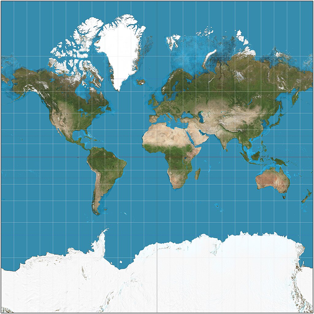
The blue curves in Figure 9.8.41 are lines with constant longitude. Longitude corresponds to an angular measurement of how far around (horizontally) on the surface of the sphere. Longitude corresponds to a shifted version of the \(\theta\) coordinate. Lines of Longitude are called meridians and the Prime Meridian corresponds to the meridian that goes through the Greenwich Naval Observatory in Greenwich, England. If you were to flatten out the surface of the globe to make the latitude and longitude lines form a rectangular grid, then you get a Mercator projection map which you may recognize. While these flat maps are convienent there is a considerable amount of distortion in these maps as you get closer to the poles. As you can see in Figure 9.8.41, the lines with constant latitude are NOT all the same length, but need to be stretched out considerably near the poles to get a rectangular grid, as in Figure 9.8.42. Measuring the distortion of area (or volume) based on these coordinates will be an important idea in the later part of Chapter 12.
A Mercator projection of the Earth with latitude and longitude lines By Strebe - Own work, CC BY-SA 3.0, https://commons.wikimedia.org/w/index.php?curid=17700069
Figure9.8.42.A Mercator projection of the Earth with latitude and longitude lines By Strebe - Own work, CC BY-SA 3.0, https://commons.wikimedia.org/w/index.php?curid=17700069
If we extended the grid of latitude and longitude to allow for multiple radii of spheres, we get a spherical coordinate grid as shown in Figure 9.8.43. You can see how visually cluttered this grid is and why you will likely not see this idea used in plotting again.
A three dimensional plot with axes labeled \(x\text{,}\)\(y\text{,}\) and \(z\text{.}\) Four groups of concentric circles shown centered at the origin with radii of 1, 2, 3, and 4. For each group of concentric cirles, there are ten circles of different sizes centered on the z-axis are shown in red. For each group of concentric cirles, there are five blue circles with center at the origin oriented through the z-axis.
The polar coordinates of a point \(P\) in \(\R^2\) are \((r,\theta)\) where \(r\) is the distance from the origin to \(P\) and \(\theta\) is the angle that the line segment from the origin to \(P\) makes with the positive \(x\)-axis. When \(P\) has rectangular coordinates \((x,y)\text{,}\) it follows that its polar coordinates are given by
The cylindrical coordinates of a point \(P\) are \((r,\theta,z)\) where \(r\) is the distance from the origin to the projection of \(P\) onto the \(xy\)-plane, \(\theta\) is the angle that the projection of \(P\) onto the \(xy\)-plane makes with the positive \(x\)-axis, and \(z\) is the vertical distance from \(P\) to the projection of \(P\) onto the \(xy\)-plane. When \(P\) has rectangular coordinates \((x,y,z)\text{,}\) it follows that its cylindrical coordinates are given by
The spherical coordinates of a point \(P\) in 3-space are \(\rho\) (rho), \(\theta\text{,}\) and \(\phi\) (phi), where \(\rho\) is the distance from \(P\) to the origin, \(\theta\) is the angle that the projection of \(P\) onto the \(xy\)-plane makes with the positive \(x\)-axis, and \(\phi\) is the angle between the positive \(z\) axis and the vector from the origin to \(P\text{.}\) When \(P\) has rectangular coordinates \((x,y,z)\text{,}\) the spherical coordinates are given by
Find an equation for the paraboloid \(z = x^{2}+y^{2}\) in spherical coordinates. (Enter rho, phi and theta for \(\rho\text{,}\)\(\phi\) and \(\theta\text{,}\) respectively.)