In single-variable calculus we learned that the derivative is useful for finding the local maxima and minima of functions and these ideas are often employed in applied settings. In particular, if a function \(f\text{,}\) such as the one shown in Figure 11.9.1 is differentiable everywhere, we know that the tangent line is horizontal at any point where \(f\) has a local maximum or minimum. Horizontal tangent lines occur when the derivative \(f'\) is zero at any such point. Thus, one way we can find possible extreme values of a given function is to first find where the derivative of the function is zero. Remember that not every point where \(f'(a)=0\) will correspond to either a local maximum or local minimum.
After finding the critical points by looking where \(f'(a)=0\) or is undefined, you may have used the derivative of \(f\) to determine whether the output of \(f\) at the critical point changed from increasing to decreasing or vice versa. This change would determine if the critical point was a local maximum, local minimum, or something else. Additionally, the concavity at the critical point could sometimes be used to classify critical points.
In multivariable calculus, we are often similarly interested in finding the greatest or least value(s) that a function may achieve. Moreover, there are many applied settings in which a quantity of interest depends on several different variables. In the preview activity below, we will use the application of elevation being a function of location (with coordinates in terms of North/South and East/West) to look at what characteristics are necessary for an input to a function of two variables to correspond with a local maximum or minimum. An emphasis of this activity is that we can only look at measurements at our current location (local information) to determine if a point is a local maximum or minimum.
In this activity, we will use a function corresponding to elevation (as a function of 2D location) to explore what properties a point corresponding to a local maximum or local minimum (of a function of two variables) must have. Similar to Activity 11.7.4, we are hiking in a foggy park and cannot see anything more than a few feet in front of us. There is nothing blocking us from walking in any particular direction, but because of the fog, we cannot see where the highest point on the mountain is. We want to try to find the top of the mountain, but we don’t have a map or trail or any line of sight to other landmarks. Our compass still works in the fog, so we can tell what direction North/South/East/West are.
We also brought a level that we can place on the ground at our feet to measure how steep the change in elevation will be in a particular direction. In other words, the level can measure the directional derivative at our current location. Conceptually, we want to understand how the measurements we can take with our level will allow us to identify when we have reached the top of the mountain.
In Activity 11.7.4, we saw how we can move toward the top of the mountain by taking steps in the “uphill” direction (the direction of greatest rate of increase for elevation). We want to state some conditions for our measurement using the level that will determine if we have reached the top of the mountain.
Suppose you are actually standing at the top of the mountain (which will correspond to a local maximum for the elevation) and you set the level at your feet in the East direction. Will the level measure that the elevation is increasing, decreasing, or constant elevation? Write a couple of sentences to justify your answer.
Remember that the level will measure the instantaneous rate of change of elevation at your current location, but will not describe what happens for a small step in the East direction.
If you are at the top of the mountain and set the level at your feet in the South direction, will the level measure that the elevation is increasing, decreasing, or constant elevation? Write a couple of sentences to justify your answer.
If you took a step to the West from the top of the mountain, should your level measurement in the West direction at your new location be increasing, decreasing, or constant elevation? Explain your reasoning.
If you took at step in any direction from the top of the mountain, should your level measurement in the direction you took the step at your new location be increasing, decreasing, or constant elevation? Explain your reasoning.
If you took at step in any direction from the lowest point in the park, should your level measurement in the forward direction (the direction in which you took the step) at your new location be increasing, decreasing, or constant elevation? Explain your reasoning.
Is it possible on your hike in the fog that you find a point where your level shows constant elevation in every direction but you are NOT at the top of the mountain or lowest point on the mountain? Explain what the the terrain would look like at this kind of location.
As you saw in the preview activity, you saw how points corresponding to local minimums and local maximums must have a zero slope in every direction and the rate of the change after taking a small step in any direction will also need to be either positive or negative (respectively). This will form the conceptual basis of our attempt to find and classify extreme points of functions of two variables.
One of the important applications of single-variable calculus is the use of derivatives to identify local extremes of functions (that is, local maxima and local minima). Using the tools we have developed so far, we can naturally extend the concept of local maxima and minima to several-variable functions.
Let \(f\) be a function of two variables \(x\) and \(y\text{.}\)
The function \(f\) has a local maximum at a point \((x_0,y_0)\) provided that \(f(x,y) \leq f(x_0,y_0)\) for all points \((x,y)\) near \((x_0,y_0)\text{.}\) In this situation we say that \(f(x_0, y_0)\) is a local maximum value.
The function \(f\) has a local minimum at a point \((x_0,y_0)\) provided that \(f(x,y) \geq f(x_0,y_0)\) for all points \((x,y)\) near \((x_0,y_0)\text{.}\) In this situation we say that \(f(x_0, y_0)\) is a local minimum value.
An absolute maximum point is a point \((x_0,y_0)\) for which \(f(x,y)\leq f(x_0,y_0)\) for all points \((x,y)\) in the domain of \(f\text{.}\) The value of \(f\) at an absolute maximum point is the maximum value of \(f\text{.}\)
An absolute minimum point is a point such that \(f(x,y) \geq f(x_0,y_0)\) for all points \((x,y)\) in the domain of \(f\text{.}\) The value of \(f\) at an absolute minimum point is the minimum value of \(f\text{.}\)
We use the term extremum point to refer to any point \((x_0,y_0)\) at which \(f\) has a local maximum or minimum. In addition, the function value \(f(x_0,y_0)\) at an extremum is called an extremal value. Figure 11.9.3 illustrates the graphs of two functions that have an absolute maximum and minimum, respectively, at the origin \((x_0,y_0) = (0,0)\text{.}\)
In single-variable calculus, we saw that the extrema of a continuous function \(f\) always occur at critical points, values of \(x\) where \(f\) fails to be differentiable or where \(f'(x) = 0\text{.}\) Said differently, critical points provide the locations where the extrema of a function may appear. Our work in Preview Activity 11.9.1 suggests that something similar happens with two-variable functions.
Suppose that a continuous function \(f\) has an extremum at \((x_0,y_0)\text{.}\) In this case, the trace \(f(x,y_0)\) has an extremum at \(x_0\text{,}\) which means that \(x_0\) is a critical value of \(f(x,y_0)\text{.}\) Therefore, either \(f_x(x_0,y_0)\) does not exist or \(f_x(x_0,y_0) = 0\text{.}\) Similarly, either \(f_y(x_0,y_0)\) does not exist or \(f_y(x_0,y_0) = 0\text{.}\) This implies that the extrema of a two-variable function occur at points that satisfy the following definition.
A critical point \((x_0,y_0)\) of a function \(f=f(x,y)\) is a point in the domain of \(f\) at which \(f_x(x_0,y_0) = 0\) and \(f_y(x_0,y_0) = 0\text{,}\) or such that one of \(f_x(x_0,y_0)\) or \(f_y(x_0,y_0)\) fails to exist.
In the analogy of Preview Activity 11.9.1, these critical points correspond to locations where our level will measure no change in elevation for every direction. How can we ensure that directional derivative will be zero in every direction? If \(\nabla f =\vec{0}\text{,}\) then \(Df_{\vu} = \vec{0}\cdot\vu = 0 \) for every direction. Geometrically, if \(\nabla f =\vec{0}\) at a point \((x_0,y_0)\text{,}\) then the tangent plane at this point will be horizontal (of the form \(z=\text{constant}\)).
We can therefore find critical points of a function \(f\) by computing partial derivatives and identifying any values of \((x,y)\) for which one of the partials doesn’t exist or for which both partial derivatives are simultaneously zero. For the latter, note that we have to solve the system of equations
In this example, we will look for the critical points of the two variable function \(f(x,y)=4x^4+y^2-16xy\text{.}\) By the definition of critical points above, we will need to solve for the \((x,y)\) points with both \(f_x\) and \(f_y\) equal to zero. Note here that there will be no points for which the partial derivatives of \(f\) will be undefined. Because \(f_x=16x^3-16y\) and \(f_y=2y-16x\text{,}\) critical points will be solutions to the system of equations
Solving the second equation for \(y\text{,}\) we get \(y=8x\text{,}\) which we can plug into the first equation to get \(16x^3-16(8x)=0\text{.}\) Factoring this equation, we get
which means our critical points must have either \(x=0\text{,}\)\(x=\sqrt{8}\text{,}\) or \(x=-\sqrt{8}\text{.}\) We can substitute each of these values back into \(y=8x\) to get the following critcal points:
For each point above, Figure 11.9.6 will show a plot of \(z=f(x,y)\) for a small region around the critical value. You can use the selector at the top of Figure 11.9.6 to choose which critical point to look at. Pay attention to how the coordinate values are changing in each case.
You can see from the plots around each of the critical points in Figure 11.9.6, that our first critical point \((x,y)=(0,0)\) will NOT be a local maximum or local minimum, but both of \((x,y)=(\sqrt{8},8\sqrt{8})\) and \((x,y)=(-\sqrt{8},-8\sqrt{8})\) will be local minimums.
The previous example shows how between minimums there does not have to be maximum (like was the case for continuous functions of one variable). We encourage you to think carefully about how possibilities can be very different than in one variable functions as we move forward.
Use Figure 11.9.7 to plot the surface near each of your critical points. You will need to put in the coordinates of your critical point as \((a,b)\) and the function you are using for \(f(x,y)\text{.}\)
Use your plots of the surfaces \(z=f(x,y)\) near your critical point to decide whether each critical point is a local maximum, a local minimum, or not an extreme point.
Subsection11.9.3Classifying Critical Points: The Second Derivative Test
While the extreme values of a continuous function \(f\) always occur at critical points, it is important to note that not every critical point leads to an extremum. Recall, for instance, \(f(x) = x^3\) from single variable calculus. We know that \(x_0=0\) is a critical point since \(f'(x_0) = 0\text{,}\) but \(x_0 = 0\) is neither a local maximum nor a local minimum of \(f\text{.}\) Geometrically, this corresponds to the tangent line \(x_0=0\) being horizontal (as seen in Figure 11.9.8) but the critical point does not correspond to a place where \(f\) is not increasing or decreasing in all directions away from the \(x_0=0\) critical point.
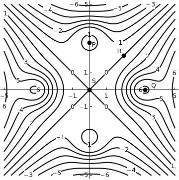
As you have seen a few times already, a similar situation can arise in a multivariable setting. Let’s look at the function \(f\) defined by \(f(x,y) = x^2 - y^2\) whose graph and contour plot are shown in Figure 11.9.9. Because \(\nabla f = \langle 2x, -2y\rangle\text{,}\) we see that the origin \((x_0,y_0)=(0,0)\) is a critical point. However, this critical point is neither a local maximum or minimum; the origin is a local minimum on the trace defined by \(y=0\text{,}\) while the origin is a local maximum on the trace defined by \(x=0\text{.}\) We call such a critical point a saddle point due to the shape of the graph near the critical point.
As in single-variable calculus, we would like to have an algebraic test to help us identify whether a critical point is a local maximum, local minimum, or neither. Recall that the Second Derivative Test for single-variable functions states that if \(x_0\) is a critical point of a function \(f\) so that \(f'(x_0)=0\) and if \(f''(x_0)\) exists, then
if \(f''(x_0) \lt 0\text{,}\) then \(x_0\) is a local maximum
The first two cases are shown geometrically in Figure 11.9.10. The inconclusive case does not necessarily mean that you have critical point like the one shown in Figure 11.9.8, but that you need more information to determine the behavior of the critical point.
If we have a critical point for a function of two variables, we will need to look at the concavity in all directions around our point. In Figure 11.9.11, you can use the dropdown box to select three different types of critical points (local maximum, local minimum, and saddle point) to examine graphically. You can also use the slider to change the direction in which the trace is plotted (in red). Notice that no matter what kind of critical point behavior is selected, the tangent plane (shown in blue) is horizontal and the trace curve (shown in red) will be tangent to the blue plane.
If you look at the local maximum critical point in Figure 11.9.11, you can use the slider to look at all directions in which you can move away from the critical point. In EVERY direction, the trace curves are concave down at our local maximum.
If you look at the local minimum critical point in Figure 11.9.11, you can use the slider to look at all directions in which you can move away from the critical point. In EVERY direction, the trace curves are concave up at our local minimum.
However, if you look at the saddle point and you change the direction that you move away from the critical point, then you will have some directions where the trace curve is concave up and some directions where the trace curve is concave down.
In order to classify our critical points, we will need to figure out if the behavior around our critical point is always concave up, always concave down, or if there is a directional dependence on concave up/down.
The good news is that we have a couple of convenient directions to look at concavity in (parallel to the \(x\) and \(y\) axes). Recall from Section 11.4 that \(f_{xx}\) and \(f_{yy}\) will measure the concavity of the traces in the \(x\) and \(y\) directions, respectively. If \(f_{xx} \gt 0\) at our critical point, then in the direction parallel to the \(x\)-axis, the trace curve will be concave up. If \(f_{xx} \lt 0\) at our critical point, then in the direction parallel to the \(x\)-axis, the trace curve will be concave down. Similar statements hold for \(f_{yy}\text{.}\)
Suppose that \(f_{xx} (a,b) \lt 0\) and \(f_{yy} \gt 0\) at a critical point \((a,b)\text{.}\) Because the concavity is different (up/down) for two different direction, the critical point \((a,b)\)must be a saddle point. Unfortunately, if \(f_{xx} (a,b) \gt 0\) and \(f_{yy} \gt 0\) at a critical point \((a,b)\text{,}\) then we do not necessarily have a local minimum, as shown in Figure 11.9.12.
As the plot in Figure 11.9.12 shows, we will need to look at the concavity in more than the coordinate axes directions. Recall from Activities 11.4.3 and Activity 11.4.4, our mixed second partial derivative \(f_{xy}\) measures the “twist” of the graph as we vary \(y\) along a particular trace where \(x\) is held constant. In the same way, \(f_{yx}\) measures how the graph twists as we vary \(x\text{.}\) For our nice functions, remember that Clairaut’s theorem tells us that \(f_{xy} = f_{yx}\text{,}\) so we will see that the amount of twisting is the same in both directions. These mixed second partial derivatives will be used to see if there is enough twist to change the concavity in the directions between the coordinate axes.
We introduce the discriminant of a function of two variables as
\begin{equation*}
D = f_{xx}(x_0,y_0) f_{yy}(x_0,y_0) - f_{xy}(x_0,y_0)^2
\end{equation*}
We claim here that if the discriminant is negative, then the concavity will change depending on direction and that if the discriminant is positive, then all directions have the same concavity. Let’s look at a few cases here.
If \(f_{xx}(x_0,y_0)\) and \(f_{yy}(x_0,y_0)\) are not both positive or both negative, then the discriminant must be negative because the second term in \(D\) is always negative. This is the case of the saddle shown above; one coordinate direction is concave up and one is concave down, thus we do not have an extreme point.
If \(f_{xx}(x_0,y_0)\) and \(f_{yy}(x_0,y_0)\) are both positive or both negative, then the first term will be positive. If our coordinate directions have the same concavity, then we will need to see if there is enough “twist” in our surface to change the concavity for directions between the coordinate axes. In other words, if \(f_{xx}(x_0,y_0) f_{yy}(x_0,y_0) \lt f_{xy}(x_0,y_0)^2\) there will be enough twist to have some direction to have different concavity from the coordinate directions.
If \(f_{xx}(x_0,y_0) f_{yy}(x_0,y_0) \gt f_{xy}(x_0,y_0)^2\text{,}\) then there will not be enough twist between the coordinate directions and every direction has the same concavity.
Suppose \((x_0,y_0)\) is a critical point of the function \(f\) for which \(f_x(x_0,y_0) = 0\) and \(f_y(x_0,y_0) = 0\text{.}\) Let \(D\) be the quantity defined by
\begin{equation*}
D = f_{xx}(x_0,y_0) f_{yy}(x_0,y_0) - f_{xy}(x_0,y_0)^2.
\end{equation*}
If \(D \gt 0\) and \(f_{xx}(x_0,y_0) \lt 0\text{,}\) then \(f\) has a local maximum at \((x_0,y_0)\text{.}\)
A key idea of the Second Partial Derivatives Test is that if the discriminant is positive, all directions have the same concavity and if the discriminant is negative, then the concavity changes from up to down depending on the direction. The last case of the Second Partial Derivatives Test is similar to the inconclusive case for the Second Derivative Test from single variable calculus.
To properly understand the origin of the Second Partial Derivatives Test, we would need to introduce a “second-order directional derivative.” If this second-order directional derivative were negative in every direction, for instance, we could guarantee that the critical point is a local maximum. A complete justification of the Second Partial Derivatives Test requires key ideas from linear algebra that are beyond the scope of this course, so instead of presenting a detailed explanation, we will accept the conceptual description given above.
As we learned in single-variable calculus, finding extremal values of functions can be particularly useful in applied settings. For instance, we can often use calculus to determine the least expensive way to construct something or to find the most efficient route between two locations. The same possibility holds in settings with two or more variables.
While the quantity of a product demanded by consumers is often a function of the price of the product, the demand for a product may also depend on the price of other products. For instance, the demand for blue jeans at a clothing store may be affected not only by the price of the jeans themselves, but also by the price of khakis.
Suppose we have two goods whose respective prices are \(p_1\) and \(p_2\text{.}\) The demand for these goods, \(q_1\) and \(q_2\text{,}\) depend on the prices as
The seller would like to set the prices \(p_1\) and \(p_2\) in order to maximize revenue. We will assume that the seller meets the full demand for each product. Thus, if we let \(R\) be the revenue obtained by selling \(q_1\) items of the first good at price \(p_1\) per item and \(q_2\) items of the second good at price \(p_2\) per item, we have
\begin{equation*}
R = p_1q_1 + p_2q_2.
\end{equation*}
Subsection11.9.4Optimization on a Restricted Domain
The Second Partials Derivative Test helps us classify critical points for a function of two variables, but it does not tell us if the function actually has an absolute maximum or minimum at each such point. For single-variable functions, the Extreme Value Theorem told us that a continuous function on a closed interval \([a, b]\) always has both an absolute maximum and minimum on that interval, and that these absolute extremes must occur at either an endpoint or at a critical point. Thus, to find the absolute maximum and minimum, we determine the critical points in the interval and then evaluate the function at these critical points and at the endpoints of the interval. A similar approach works for functions of two variables.
For functions of two variables, closed and bounded regions play the role that closed intervals did for functions of a single variable. A closed region is a region that contains its boundary (the unit disk \(x^2+y^2 \leq 1\) is closed, while its interior \(x^2+y^2 \lt 1\) is not, for example), while a bounded region is one that does not stretch to infinity in any direction. Just as for functions of a single variable, continuous functions of several variables that are defined on closed, bounded regions must have absolute maxima and minima in those regions.
Let \(f= f(x,y)\) be a continuous function on a closed and bounded region \(R\text{.}\) Then \(f\) has an absolute maximum and an absolute minimum in \(R\text{.}\)
If you wanted to find the highest point in your state, you need to look up the elevations for the tops of the hills/mountains and compare those values to the elevation along the borders. Note that the elevation along a border of your state is a one-dimensional maximization problem and you can use your tools from single variable calculus.
The absolute extremes must occur at either a critical point in the interior of \(R\) or at a boundary point of \(R\text{.}\) We therefore must test both possibilities, as we demonstrate in the following example.
For this example we will be looking to find the maximum and minimum temperature values on a heated circular plate. The plate has a 1 meter radius and we will measure the location on the plate from the center. The domain \(R=\{(x,y):x^2+y^2 \leq 1\}\) of our temperature function is a closed and bounded region, as shown in Figure 11.9.15.
Because our domain for \(T\) is closed and bounded, the Extreme Value Theorem guarantees that \(T\) has an absolute maximum and minimum on the plate. The graph of \(T\) over its domain \(R\) is shown in Figure 11.9.16. We will find the hottest and coldest points on the plate.
If the absolute maximum or minimum occurs inside the disk, then the absolute extreme point will be at a critical point, so we begin by looking for critical points inside the disk. To do this, notice that critical points are given by the conditions \(T_x= 4x=0\) and \(T_y=2y - 1=0\text{.}\) This means that there is one critical point of the function at the point \((x_0,y_0) =(0,1/2)\text{,}\) which lies inside the disk.
We now find the hottest and coldest points on the boundary of the disk, which is the circle of radius 1. As we have seen, the points on the unit circle can be parametrized as
To find the hottest and coldest points on the boundary, we look for the critical points of this single-variable function on the interval \(0\leq t\leq 2\pi\text{.}\) We have
This shows that we have critical points when \(\cos(t) = 0\) or \(\sin(t) = -1/2\text{.}\) This occurs when \(t=\pi/2\text{,}\)\(3\pi/2\text{,}\)\(7\pi/6\text{,}\) and \(11\pi/6\text{.}\) Since we have \(x(t) = \cos(t)\) and \(y(t) = \sin(t)\text{,}\) the corresponding points are
We now have a list of candidates for the hottest and coldest points: the critical point in the interior of the disk and the critical points on the boundary. We find the hottest and coldest points by evaluating the temperature at each of these points, and find that
So the maximum temperature on the disk \(x^2+y^2\leq 1\) is \(\frac{9}{4}\text{,}\) which occurs at the two points \(\left(\pm\frac{\sqrt{3}}{2},-\frac{1}{2}\right)\) on the boundary, and the minimum value of \(T\) on the disk is \(-\frac{1}{4}\) which occurs at the critical point \(\left(0,\frac{1}{2}\right)\) in the interior of \(R\text{.}\)
From this example, we see that we use the following procedure for determining the absolute maximum and absolute minimum of a function on a closed and bounded domain.
Step 1:.
Find all critical points of the function in the interior of the domain.
Find all the critical points of the function on the boundary of the domain. Working on the boundary of the domain reduces this part of the problem to one or more single variable optimization problems. Note that there may be endpoints on portions of the boundary that need to be considered.
The maximum value of the function is the largest value obtained in Step 3, and the minimum value of the function is the smallest value obtained in Step 3.
Let \(f(x,y) = x^2-3y^2-4x+6y\) with triangular domain \(R\) whose vertices are at \((0,0)\text{,}\)\((4,0)\text{,}\) and \((0,4)\text{.}\) The domain \(R\) appears in Figure 11.9.17. In this activity, we will go through the steps to find the absolute maximum and minimum of \(f\) on \(R\text{.}\)
To find the extrema of a function \(f=f(x,y)\text{,}\) we first find the critical points, which are points where one of the partials of \(f\) fails to exist, or where \(f_x = 0\) and \(f_y=0\text{.}\)
If \(f\) is defined on a closed and bounded domain, we find the absolute maxima and minima by finding the critical points in the interior of the domain, finding the critical points on the boundary, and testing the value of \(f\) at both sets of critical points.
There are several critical points to be listed. List them lexicographically, that is in ascending order by \(x\)-coordinates, and for equal \(x\)-coordinates in ascending order by \(y\)-coordinates (e.g., (1,1),(1,10), (2, -1), (2, 3) is a correct order)
Explain why \(f\) must have a global minimum at some point in \(R\) (note that \(R\) is unbounded---how does this influence your explanation?). Then find the global minimum.
Each of the following functions has at most one critical point. Graph a few level curves and a few gradients and, on this basis alone, decide whether the critical point is a local maximum, a local minimum, a saddle point, or that there is no critical point.
List the minimum/maximum values as well as the point(s) at which they occur. If a min or max occurs at multiple points separate the points with commas.
(a) Supposed that at \((5,1)\text{,}\) we know that \(f_x=f_y=0\) and \(f_{xx} \lt 0\text{,}\)\(f_{yy} \lt 0\text{,}\) and \(f_{xy} = 0\text{.}\) What can we conclude about the behavior of this function near the point \((5,1)\text{?}\)
(b) Supposed that at \((6,-1)\text{,}\) we know that \(f_x=f_y=0\) and \(f_{xx} \lt 0\text{,}\)\(f_{yy} > 0\text{,}\) and \(f_{xy} = 0\text{.}\) What can we conclude about the behavior of this function near the point \((6,-1)\text{?}\)
(c) Supposed that at \((8,-2)\text{,}\) we know that \(f_x=f_y=0\) and \(f_{xx} = 0\text{,}\)\(f_{yy} \lt 0\text{,}\) and \(f_{xy} > 0\text{.}\) What can we conclude about the behavior of this function near the point \((8,-2)\text{?}\)
Hint: By symmetry, you can restrict your attention to the first octant (where \(x, y, z \ge 0\)), and assume your volume has the form \(V =
8xyz\text{.}\) Then arguing by symmetry, you need only look for points which achieve the maximum which lie in the first octant.
Design a rectangular milk carton box of width \(w\text{,}\) length \(l\text{,}\) and height \(h\) which holds \(498 \text{ cm}^3\) of milk. The sides of the box cost \(3 \ \text{cents/cm}^2\) and the top and bottom cost \(4\ \text{cents/cm}^2\text{.}\) Find the dimensions of the box that minimize the total cost of materials used.
Respond to each of the following prompts to solve the given optimization problem.
Let \(f(x,y) = \sin(x)+\cos(y)\text{.}\) Determine the absolute maximum and minimum values of \(f\text{.}\) At what points do these extreme values occur?
Determine the absolute maximum and absolute minimum of \(f(x,y) = 2 + 2x + 2y - x^2 - y^2\) on the triangular plate in the first quadrant bounded by the lines \(x = 0\text{,}\)\(y = 0\text{,}\) and \(y = 9-x\text{.}\)
Determine the absolute maximum and absolute minimum of \(f(x,y) = 2 + 2x + 2y - x^2 - y^2\) over the closed disk of points \((x,y)\) such that \((x-1)^2 + (y-1)^2 \le 1\text{.}\)
If a continuous function \(f\) of a single variable has two critical numbers \(c_1\) and \(c_2\) at which \(f\) has relative maximum values, then \(f\) must have another critical number \(c_3\text{,}\) because “it is impossible to have two mountains without some sort of valley in between. The other critical point can be a saddle point (a pass between the mountains) or a local minimum (a true valley).” (From Calculus in Vector Spaces by Lawrence J. Corwin and Robert H. Szczarb.) Consider the function \(f\) defined by \(f(x,y) = 4x^2e^y -2x^4 -e^{4y}\text{.}\) (From Ira Rosenholz in the Problems Section of the Mathematics Magazine, Vol. 60 NO. 1, February 1987.) Show that \(f\) has exactly two critical points, and that \(f\) has relative maximum values at each of these critical points. Explain how this function \(f\) illustrates that it really is possible to have two mountains without some sort of valley in between. Use appropriate technology to draw the surface defined by \(f\) to see graphically how this happens.
If a continuous function \(f\) of a single variable has exactly one critical number with a relative maximum at that critical point, then the value of \(f\) at that critical point is an absolute maximum. In this exercise we see that the same is not always true for functions of two variables. Let \(f(x,y) = 3xe^y-x^3-e^{3y}\) (from “The Only Critical Point in Town” Test by Ira Rosenholz and Lowell Smylie in the Mathematics Magazine, VOL 58 NO 3 May 1985.). Show that \(f\) has exactly one critical point, has a relative maximum value at that critical point, but that \(f\) has no absolute maximum value. Use appropriate technology to draw the surface defined by \(f\) to see graphically how this happens.
A manufacturer wants to procure rectangular boxes to ship its product. The boxes must contain 20 cubic feet of space. To be durable enough to ensure the safety of the product, the material for the sides of the boxes will cost $0.10 per square foot, while the material for the top and bottom will cost $0.25 per square foot. In this activity we will help the manufacturer determine the box of minimal cost.
What quantities are constant in this problem? What are the variables in this problem? Provide appropriate variable labels. What, if any, restrictions are there on the variables?
Your formula in part (b) might be in terms of three variables. If so, find a relationship between the variables, and then use this relationship to write \(C\) as a function of only two independent variables.
A rectangular box with length \(x\text{,}\) width \(y\text{,}\) and height \(z\) is being built. The box is positioned so that one corner is stationed at the origin and the box lies in the first octant where \(x\text{,}\)\(y\text{,}\) and \(z\) are all positive. There is an added constraint on how the box is constructed: it must fit underneath the plane with equation \(x + 2y + 3z = 6\text{.}\) In fact, we will assume that the corner of the box “opposite” the origin must actually lie on this plane. The basic problem is to find the maximum volume of the box.
Sketch the plane \(x + 2y + 3z = 6\text{,}\) as well as a picture of a potential box. Label everything appropriately.
Explain how you can use the fact that one corner of the box lies on the plane to write the volume of the box as a function of \(x\) and \(y\) only. Do so, and clearly show the formula you find for \(V(x,y)\text{.}\)
Find all critical points of \(V\text{.}\) (Note that when finding the critical points, it is essential that you factor first to make the algebra easier.)
Without considering the current applied nature of the function \(V\text{,}\) classify each critical point you found above as a local maximum, local minimum, or saddle point of \(V\text{.}\)
Now suppose that we instead stipulated that, while the vertex of the box opposite the origin still had to lie on the plane, we were only going to permit the sides of the box, \(x\) and \(y\text{,}\) to have values in a specified range (given below). That is, we now want to find the maximum value of \(V\) on the closed, bounded region
\begin{equation*}
\frac{1}{2} \le x \le 1, \ \ 1 \le y \le 2.
\end{equation*}
Find the maximum volume of the box under this condition, justifying your answer fully.
Let \(x\text{,}\)\(y\text{,}\) and \(z\) be the length, width, and height (in inches) of a carry on bag. In this problem we find the dimensions of the bag of largest volume, \(V = xyz\text{,}\) that satisfies the second restriction. Assume that we use all 45 inches to get a maximum volume. (Note that this bag of maximum volume might not satisfy the third restriction.)
Write the volume \(V=V(x,y)\) as a function of just the two variables \(x\) and \(y\text{.}\)
Find the maximum value of \(V\) on the boundary of the region \(R\text{,}\) and then determine the dimensions of a bag with maximum volume on the entire region \(R\text{.}\) (Note that most carry-on bags sold today measure \(22\) by \(14\) by \(9\) inches with a volume of \(2772\) cubic inches, so that the bags will fit into the overhead bins.)
According to The Song of Insects by G.W. Pierce (Harvard College Press, 1948) the sound of striped ground crickets chirping, in number of chirps per second, is related to the temperature. So the number of chirps per second could be a predictor of temperature. The data Pierce collected is shown in Table 11.9.19., where \(x\) is the (average) number of chirps per second and \(y\) is the temperature in degrees Fahrenheit.
A scatterplot of the data would show that, while the relationship between \(x\) and \(y\) is not exactly linear, it looks to have a linear pattern. It could be that the relationship is really linear but experimental error causes the data to be slightly inaccurate. Or perhaps the data is not linear, but only approximately linear.
If we want to use the data to make predications, then we need to fit a curve of some kind to the data. Since the cricket data appears roughly linear, we will fit a linear function \(f\) of the form \(f(x) = mx+b\) to the data. We will do this in such a way that we minimize the sums of the squares of the distances between the \(y\) values of the data and the corresponding \(y\) values of the line defined by \(f\text{.}\) This type of fit is called a least squares approximation. If the data is represented by the points \((x_1,y_1)\text{,}\)\((x_2,y_2)\text{,}\)\(\ldots\text{,}\)\((x_n,y_n)\text{,}\) then the square of the distance between \(y_i\) and \(f(x_i)\) is \((f(x_i)-y_i)^2 = (mx_i+b-y_i)^2\text{.}\) So our goal is to minimize the sum of these squares, of minimize the function \(S\) defined by
(Hint: Don’t be daunted by these expressions, the system \(S_m(m,b) = 0\) and \(S_b(m,b) = 0\) is a system of two linear equations in the unknowns \(m\) and \(b\text{.}\) It might be easier to let \(r=\sum_{i=1}^n x_i^2\text{,}\)\(s=\sum_{i=1}^n x_i\text{,}\)\(t = \sum_{i=1}^n y_i\text{,}\) and \(u = \sum_{i=1}^n x_iy_i\) and write your equations using these constants.)
Use the Second Derivative Test to explain why the critical point gives a local minimum. Can you then explain why the critical point gives an absolute minimum?
Use the formula from part (b) to find the values of \(m\) and \(b\) that give the line of best fit in the least squares sense to the cricket data. Draw your line on the scatter plot to convince yourself that you have a well-fitting line.