Section 11.2 Functions of Several Variables

Notes to the Instructor and Dependencies.

This section expects students to have familiarity with our discussion of 3D coordinates and fundamental planes in SectionΒ 9.2 and properties of functions from precalculus (domain, range, etc.). This section can probably be covered in in a single class meeting but students will need to practice with the ideas of traces and contour plots since those will be used throughout the next three chapters.
There are a variety of activities in this section that will allow an instructor to select how much algebraic versus conceptual coverage they would prefer. Some instructors may skip elements like domain and range and would not need to do ActivityΒ 11.2.2. ActivityΒ 11.2.3 introduces users to the spreadsheet version of multivariable functions that will used in application settings for the next couple of chapters. ActivityΒ 11.2.4 helps users to connect work with traces and practice drawing surfaces. There are a few different activities you can select from related to contours and how to visualize surfaces.

Subsection 11.2.1 Introduction

In this section, we will start our work with (scalar valued) multivariable functions by looking at several basic elements of these type of functions, such as domain, range, different presentations, and how to plot these functions. Our preview activity will use a finance example to get you used to the notation and descriptions of different aspects of functions of several variables.


Preview Activity 11.2.1.

Suppose you invest money in an account that pays 5% interest compounded continuously. If you have an initial investment of \(P\) dollars in the account, then \(A\text{,}\) the amount of money in the account after \(t\) years is given by
\begin{equation*} A = Pe^{0.05t}. \end{equation*}
The variables \(P\) and \(t\) are independent of each other, so using functional notation we write
\begin{equation*} A(P,t) = Pe^{0.05t}. \end{equation*}
(a)
Find the amount of money in the account after 7 years if you originally invest 1000 dollars.
(b)
Evaluate \(A(5000,8)\text{.}\) Write a sentence to explain what this calculation represents.
(c)
Now consider only the situation where the amount invested is fixed at 1000 dollars. Calculate the amount of money in the account after \(t\) years as indicated in the table below. Round payments to the nearest penny.
Duration (in years) 2 3 4 5 6
Amount (dollars)
(d)
Now consider the situation where we want to know the amount of money in the account after 10 years given various initial investments. Calculate the amount of money in the account as indicated in the table below. Round payments to the nearest penny.
Initial investment (dollars) 500 1000 5000 7500 10000
Amount (dollars)
(e)
Describe as best you can what combinations of initial investments and time will result in an account containing $10,000.

Subsection 11.2.2 Functions of Several Variables

Up to this chapter, we have primarily been concerned with functions of a single variable. Remember that a function is a rule that assigns exactly one output for each allowed input. For instance, the rule that assigns a student ID number to each student at your school is a function because each student (input) gets assigned one and only one ID number. The rule that assigns the classrooms for your courses this semester is not a function because you likely have more than one classroom (multiple outputs) for each student (a single input).
We saw the behavior of a function in Preview ActivityΒ 11.2.1, where each pair of inputs, \((P,t)\text{,}\) produces a single output \(A(P,t)\text{.}\) Additionally, the values of the two variables \(P\) and \(t\) did not depend on one another. That is, we could choose any value of \(P\) without limiting what value \(t\) might have, and we could select any value of \(t\) to use without regard to what value \(P\) might have. For that reason we say that the variables \(t\) and \(P\) are independent of each other. Thus, we call \(A = A(P,t)\) a function of the two independent variables \(P\) and \(t\text{.}\) This is the key idea in defining a function of two independent variables.

Definition 11.2.1.

A function \(f\) of two independent variables is a rule that assigns to each ordered pair \((x,y)\) in some set \(D\) exactly one real number \(f(x,y)\text{.}\)
There is no reason to restrict ourselves to functions of only two variables; we can use any number of variables we like. For example,
\begin{equation*} f(x,y,z) = x^2 - 2xz + \cos(y) \end{equation*}
defines \(f\) as a function of the three variables \(x\text{,}\) \(y\text{,}\) and \(z\text{.}\) In general, a function of \(n\) independent variables is a rule that assigns to an ordered \(n\)-tuple \((x_1, x_2, \ldots, x_n)\) in some set \(D\) exactly one real number.
 1 
You may notice that we use variable names like \(x,y,z\) when using three variables but when there are more than three variables, it will be convenient to index the variables like \(x_i\) so that we can refer to the variables by index. For example the fifth variable in \((x_1, x_2, \ldots, x_n)\) will be \(x_5\) and the last two variables will be \(x_{n-1}\) and \(x_n\text{.}\)
As with functions of a single variable, it is important to understand the set of inputs for which the function is defined.

Definition 11.2.2.

The domain of a function \(f\) is the set of all inputs for which the function is defined.
The range of a function \(f\) is the set of all actual outputs for the function.
Recall that common ways for scalar functions to not be defined for a particular input include:
  • dividing by zero,
  • taking the square root of negative numbers, and
  • restricted domains from other functions like \(\arcsin\) or logarithms.
For multivariable functions, we have similar phenomena to consider.

Example 11.2.3.

In this example, we will look at the domain and range of a couple of multivariable functions.

(a)

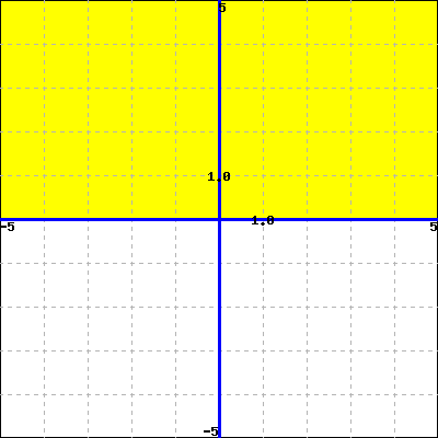
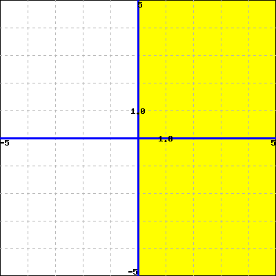
Let \(f(x,y)=\sqrt{xy}\text{.}\) For the domain of \(f\) we can only use \((x,y)\)-inputs where \(\sqrt{xy}\) is defined. This requires that \(xy\) be nonnegative. We will use set-builder notation to describe this domain. The domain of \(f\) is \(\{(x,y)\in\mathbb{R}^2\mid xy \geq 0\}\text{.}\) This notation is read as β€œthe set of \((x,y)\) coordinates in the cartesian plane such that \(x\) times \(y\) is greater than or equal to zero”. Set builder notation is flexible because this follows the form \(\{\text{kind of objects}\mid \text{conditions on objects}\}\text{.}\) The symbol \(|\) is read as β€œsuch that”. Note that the domain of \(f\) does not say that \(x\) and \(y\) are both nonnegative (quadrant I), but rather that the product of \(x\) and \(y\) needs to be nonnegative (quadrants I and III).
described in detail following the image
A plot highlighting the first and third quadrants which includes both coordinate axes
Figure 11.2.4. A plot of the domain of \(f(x,y)=\sqrt{xy}\)
When we consider the range of \(f(x,y)=\sqrt{xy}\) we need to think about what values can be outputs of \(f\text{.}\) You may be tempted to say that outputs are scalars, so the range should be all real numbers, \(\mathbb{R}\text{.}\) However, there is no way to get a negative output for \(f\text{.}\) Thus, not all real numbers are actual outputs of \(f\text{.}\) Instead, the range of \(f\) will be the interval \([0,\infty)\) because those are the values that \(f\) actually outputs. (Specifically, for any nonnegative real number \(c\text{,}\) \(f(c,c) = \sqrt{cc} = c\text{.}\))

(b)

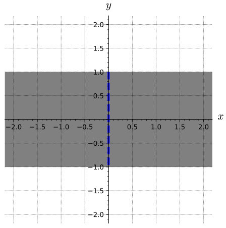
We now consider the domain and range of \(g(x,y)=\frac{\arcsin(y)}{2x}\text{.}\) First we need to recall the domain and range of the arcsine function are \([-1,1]\) and \([-\frac{\pi}{2},\frac{\pi}{2}]\text{,}\) respectively. Thus, the only valid inputs to \(g\) must have \(y\)-values in the interval \([-1,1]\) and we must also have \(x\neq0\) because we cannot divide by zero. Thus the domain of \(g\) is \(\{(x,y)\in\mathbb{R}^2 \mid x \neq 0 \text{ and } -1 \leq y \leq 1\}\text{.}\)
described in detail following the image
A plot with the horizontal band having \(-1\leq y\leq 1\) shaded. The portion of this region with \(x=0\) is marked with a dashed line.
Figure 11.2.5. A plot of the domain of \(g(x,y)=\frac{\arcsin(y)}{2x}\)
The range of arcsine is \([-\frac{\pi}{2},\frac{\pi}{2}]\) but since the output of \(g\) will be \(\frac{\arcsin(y)}{2x}\text{,}\) the range of \(g\) will be \(\mathbb{R}\text{,}\) all real numbers. For example, the input \((\frac{\pi}{4a},1)\) will be sent to \(a\) for any value of \(a\neq 0\) and \(g(0,1)=0\text{.}\)


Subsection 11.2.3 Representing Functions of Two Variables

Algebraic rules.

You have already seen one representation of a function of several variables: the algebraic notation \(f(x,y)=\sqrt{xy}\text{,}\) which shows an algebraic rule to find the output of the function \(f\) for given input values \(x\) and \(y\text{.}\) This kind of representation is convenient to use with algebraic rules for derivatives or for computing the output of a function given particular inputs. The drawback to this representation is that you need a lot of intuition about the type of function being used to understand how the output changes over a range of values.

Tables.

One of the techniques we use to study functions of one variable is to create a table of values. We can do the same for functions of two variables, except that our tables must allow us to keep track of both input variables. We can do this with a two-dimensional table, where we list the \(x\)-values down the first column and the \(y\)-values across the first row.
As an example, suppose we launch a projectile (perhaps by hitting a golf ball with a golf club) from ground level. Under ideal conditions, by which we mean ignoring wind resistance, spin, or any other forces except the force of gravity, the horizontal distance the object travels before hitting the ground depends on the initial velocity \(x\) the object is given, and the angle \(y\) at which it is launched. If we let \(f\) represent the horizontal distance the object travels, then \(f\) is a function of the two variables \(x\) and \(y\text{,}\) and we represent \(f\) in functional notation by
\begin{equation*} f(x,y) = \frac{x^2 \sin(2 y)}{g}\text{,} \end{equation*}
where \(g\) is the acceleration due to gravity.
 2 
Note that \(g\) is constant, \(9.8\) meters per second squared or \(32\) feet per second squared.
To create a table of values for \(f\text{,}\) we list the \(x\)-values down the first column and the \(y\)-values across the first row. The value \(f(x,y)\) is displayed in the location where the \(x\) row intersects the \(y\) column, as shown in TableΒ 11.2.6, where we measure \(x\) in feet per second and \(y\) in radians. For example, \(f(75,0.8)=175.7\) is shown in the table by looking at the value in the row with \(x=75\) and column corresponding to \(y=0.8\text{.}\)


Activity 11.2.3.

Complete TableΒ 11.2.6 by filling in the missing values of the function \(f\text{.}\) Round entries to the nearest tenth.
Table 11.2.6. Values of \(f(x,y) = \displaystyle \frac{x^2 \sin(2y)}{g}\) with \(g=32 \text{ft/s}^2\)
\(x \Downarrow \backslash y\Rightarrow\) \(0.4\) \(0.6\) \(0.8\) \(1.0\) \(1.2\)
50 56.0 72.8 78.1 71.0
75 163.8 175.7 159.8 118.7
100 224.2 291.3 312.4 284.2 211.1
125 350.3 455.1 444.0 329.8
150 504.4 655.3 702.8 639.3 474.9
175 686.5 892.0 956.6 870.2
Representing a function with a table should reinforce the idea that each of the two independent values for the input variables will have a corresponding output value. However, when looking at a large table of values, it is normal to feel that this representation provides little insight into the relationship described by the function. Additionally, the table is only useful for the input values selected in the rows and columns. While this may seem like a very limited use case, many applied problems involve tables like this because an algebraic function can be extremely difficult to find for every case and it can be very expensive to test many input values to obtain the corresponding output values. You likely have already used spreadsheets to organize information in a multivariable setting like this.

Graphs.

If \(f\) is a function of a single variable \(x\text{,}\) then we define the graph of \(f\) to be the set of points of the form \((x,f(x))\text{,}\) where \(x\) is in the domain of \(f\text{.}\) We then plot these points using the coordinate axes in order to visualize the graph. We can do a similar thing with functions of several variables. TableΒ 11.2.6 identifies points of the form \((x,y,f(x,y))\text{,}\) and we define the graph of \(f\) to be the set of these points in \(\R^3\text{.}\)

Definition 11.2.7.

The graph of a function \(f = f(x,y)\) is the set of points of the form \((x,y,f(x,y))\text{,}\) where the point \((x,y)\) is in the domain of \(f\text{.}\)
We also often refer to the graph of a function \(f\) of two variables as the surface generated by \(f\text{.}\) Points of the form \((x,y,f(x,y))\) are in three dimensions. If we consider the graph of the projectile distance function defined by \(f(x,y) = \frac{x^2 \sin(2y)}{g}\text{,}\) then the function \(f\) is continuous in both variables. When these points are plotted in the rectangular coordinate system, the points form a surface in three-dimensional space. The graph of the distance function \(f\) is shown in FigureΒ 11.2.8.
A plot of a curved surface that this is u-shaped along constant values of one coordinate and increases parabolically as that the other horizontal coordinate is increased.
Figure 11.2.8. The projectile distance surface given by \(z=f(x,y) = \frac{x^2 \sin(2y)}{g}\)
There are many graphing tools available for drawing three-dimensional surfaces as indicated in the Preface and most of the in-text three-dimensional graphics are generated by SageMath. Since we will be able to visualize graphs of functions of two independent variables using plots in three dimensions, but not functions of more than two variables, we will primarily deal with functions of two variables in this chapter. It is important to note, however, that the techniques we develop apply to functions of any number of variables and we will highlight these extensions to higher dimensions in SectionΒ 11.9.
You may have noticed that we used the notation \(z=f(x,y)\) in the caption to FigureΒ 11.2.8, which is explicitly saying that we are viewing the \(z\)-coordinate in our plot as the output of the function \(f\text{.}\) In other words, only \((x,y,z)\) points of the form \((x,y,f(x,y))\) are part of the graph plotted. In some situations, it may be advantageous to express a graph of interest using a function with some input and output roles in a different configuration of coordinates. For instance, the surface shown in FigureΒ 11.2.9 cannot be expressed with the \(z\)-coordinate as a function of the \(x\)- and \(y\)-coordinates because there would be more than one \(z\)-coordinate associated to inputs such as \((x,y)=(0,1)\text{,}\) as highlighted by the red points in the figure. The points on this surface can be expressed with \(y\) as a function of \(x\) and \(z\text{,}\) however! Specifically \(y=g(x,z) = \frac{x^2}{5}+z^2\text{.}\) We will typically look at examples where \(z\) is expressed as a function of \(x\) and \(y\text{,}\) but you should think carefully if it is advantageous to consider a different coordinate view.
A bowl shaped surface is shown opening to the side. A red segment is drawn through this surface changing only in the vertical coordinate. The two points at which this red segment intersects the surface are highlighted in red and the segment is labeled β€œSame \((x,y)\) value”.
Figure 11.2.9. The surface given by \(y=g(x,z) = \frac{x^2}{5}+z^2\)

Subsection 11.2.4 Traces

When studying functions of several variables, we are often interested in how each individual variable affects the function while the other variable is fixed. In Preview ActivityΒ 11.2.1, we saw that the amount of money in an account depends on the amount initially invested and the duration of the investment. However, if we fix the initial investment, the amount of money in the account depends only on the duration of the investment, and if we fix the duration of the investment, then the amount of money in the account depends only on the initial investment. This idea of keeping one variable constant while we allow the other to change will be an important tool for us when studying functions of several variables.
 3 
This will be the first of many times we will employ the following approach
described in detail following the image
A two panel meme with a picture of a man extending his hand with a stop gesture in the top left and the textβ€œThree-dimensional problems” in the top right. A picture of the man pointing his finger appears in the bottom left with the text β€œThree One-dimensional Problems” to the lower right.
As another example, consider again the projectile distance function \(f\) defined by
\begin{equation*} f(x,y) = \frac{x^2 \sin(2y)}{g}\text{,} \end{equation*}
where \(x\) is the initial velocity of an object in feet per second, \(y\) is the launch angle in radians, and \(g\) is the acceleration due to gravity (32 feet per second squared). If we hold the launch angle constant at \(y=0.6\) radians, we can consider \(f\) a function of the initial velocity alone. In this case we have
\begin{equation*} f(x) = \frac{x^2}{32}\sin(2\cdot 0.6)\text{.} \end{equation*}
Similarly, if we fix the initial velocity at 150 feet per second, we can consider the projectile distance as a function of the launch angle only. In this case we have
\begin{equation*} f(y) = \frac{150^2 \sin(2y)}{32}\text{.} \end{equation*}
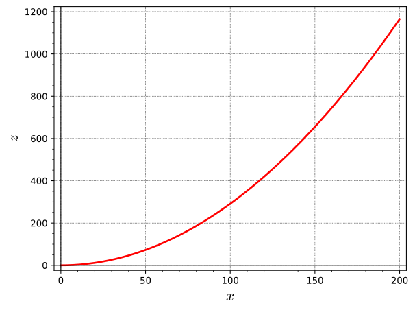
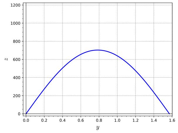
In FigureΒ 11.2.10, we show two plots. FigureΒ 11.2.10(a) shows what happens when fixing \(y=0.6\text{,}\) while FigureΒ 11.2.10(b) shows the two-dimensional graph obtained by fixing \(x=150\text{.}\)
described in detail following the image
A two dimensional plot with the horizontal coordinate labeled \(x\) and shown from 0 to 200. The vertical coordinate is labeled \(z\) and is shown from 0 to 1200. A parabola is drawn from the bottom left at (0,0) to the top right.
(a) A plot of \(f(x,0.6) = \frac{x^2}{32}\sin(2\cdot 0.6)\)
described in detail following the image
A two dimensional plot with the horizontal coordinate labeled \(y\) and is shown from 0 to 1.6. The vertical coordinate is labeled \(z\) and is shown from 0 to 1200. A parabola drawn in blue is facing down with vertex at \((\pi/4,700)\text{.}\)
(b) A plot of \(f(150,y) = \frac{150^2 \sin(2y)}{32}\)
Figure 11.2.10. Plots illustrating values of \(f\) when one variable is fixed
We can plot the curve from FigureΒ 11.2.10(a) on the surface by tracing out the points on the surface when \(y = 0.6\text{,}\) as shown in red in FigureΒ 11.2.11. The formula for \(f(x,0.6)\) shows that \(f\) is quadratic in the \(x\)-direction. More descriptively, as we increase the launch velocity while keeping the launch angle constant, the horizontal distance the object travels increases proportional to the square of the initial velocity.
We can plot the curve from FigureΒ 11.2.10(b) on the surface by tracing out the points on the surface when \(x=150\text{,}\) as shown in blue in FigureΒ 11.2.11. The formula for \(f(150,y)\) shows that \(f\) is sinusoidal in the \(y\)-direction. More descriptively, as we increase the launch angle while keeping the initial velocity constant, the horizontal distance traveled by the object is proportional to the sine of twice the launch angle.
A three dimensional plot of a curved surface that this is u-shaped along constant values of one coordinate and increases parabolically as that the other horizontal coordinate is increased. On the lower corner of this curved surface are drawn three mutually perpendicular line segments labeled \(x\text{,}\) \(y\text{,}\) and \(z\) signifying origin. In the direction of the segment labeled y from the origin, there is a two dimensional flat grid labeled \(x\) horizontally and \(z\) vertically. A branch of a parabola is shown in red from the bottom left of this grid to the top right. This red curve is copied along the curved surface along a direction that is parallel to the segment labeled x (from the origin). In the direction of the segment labeled x from the origin, there is a two dimensional flat grid labeled \(y\) horizontally and \(z\) vertically. A parabola is shown in blue pointing downward on this grid with a vertex about half way up the grid. This blue curve is copied along the curved surface along a direction that is parallel to the segment labeled y (from the origin).
Figure 11.2.11. The surface given by \(z=f(x,y) = \frac{x^2 \sin(2y)}{g}\) with traces \(y=0.6\) (in red) and \(x=150\) (in blue)
The curves we define when we fix one of the independent variables in our two-variable function are called traces. In FigureΒ 11.2.11, we have made a copy of the trace off to the side of the figure so you can see each trace as a curve on the proper two-dimensional slice. FigureΒ 11.2.10 illustrates these traces as two-dimensional plots.

Definition 11.2.12.

A trace in the \(x\)-direction of a function \(f\) of the independent variables \(x\) and \(y\) is a curve of the form \(z = f(x,c)\text{,}\) where \(c\) is a constant. Similarly, a trace in the \(y\)-direction of a function \(f\) of the two independent variables \(x\) and \(y\) is a curve of the form \(z = f(c,y)\text{,}\) where \(c\) is a constant.
Understanding trends in the behavior of functions of two variables can be challenging, as can sketching their graphs; traces help us with both of these tasks.


Activity 11.2.4.

In this activity, we investigate the use of traces to better understand a function through both tables and graphs.
(a)
Identify the \(y = 0.6\) trace for the distance function \(f\) defined by \(f(x,y) = \frac{x^2 \sin(2y)}{g}\) by highlighting or circling the appropriate cells in TableΒ 11.2.6. Write a sentence to describe the behavior of the function along this trace.
(b)
Identify the \(x = 150\) trace for the distance function by highlighting or circling the appropriate cells in TableΒ 11.2.6. Write a sentence to describe the behavior of the function along this trace.
(c)
In the next several parts, we will be looking at using traces to help us draw an accurate plot of the surface given by \(z=g(x,y)=yx^2\text{.}\) As a first step, find the equation for the \(y=1\) trace of \(z=g(x,y)=yx^2\) and draw a graph of the \(y=1\) trace on the corresponding face in FigureΒ 11.2.13.
A three dimensional plot of sides of a box shown in gray. The sides of this box are shown with a grid from negative one to one in both the horizontal and vertical coordinates.
Figure 11.2.13. A bounding box for the region with \(-1 \leq x,y,z \leq 1\)
(e)
Draw a few traces (at least three more) that correspond to values in the middle of the plot to fill in a plot of the surface given by \(z=x^2y\text{.}\)
ActivityΒ 11.2.4 shows how drawing traces on a plot of a surface can give the viewer more information about the orientation of the graph. In FigureΒ 11.2.14 you can see a plot of the surface generated in our projectile motion example. Without any of the traces drawn on the surface, it is difficult to understand the shape of the surface, and it would be even harder if not for the shading on the computer-generated graphics. You can click on the check box at the top of the figure to add traces to the plot. Notice how much easier it is to distinguish the shape of the surface at different points!
An interactive three dimensional plot of a curved surface shown in light gray that this is u-shaped along constant values of one coordinate and increases parabolically as that the other horizontal coordinate is increased. A checkbox at the top of the plot will add a set of grid lines along the surface that allow the user to see the surface through more than shading of the surface.
Figure 11.2.14. A plot of the distance surface with or without traces for perspective
When drawing plots by hand, it is important to use parallel structure to make it easier for the viewer to orient the traces as being in a direction parallel to one of the coordinate axes. It may take time for you to feel confident drawing these kinds of features by hand. However, visual representations of surfaces and their features will be very valuable in our work for the next several chapters. We will continue to provide tips and suggestions to help you with your visualizations along the way.

Subsection 11.2.5 Contour Maps and Level Curves

As you saw earlier in this section, traces give important information about what a slice of a surface looks like when holding one of the inputs constant. This corresponds to looking at the intersection of a fundamental plane of the form \(x=a\) or \(y=b\) with the surface given by \(z=f(x,y)\text{.}\) These fundamental planes are oriented vertically when we consider a conventional right-handed coordinate system. In this section, we will explore the intersection of a surface given by \(z=f(x,y)\) with a fundamental plane of the form \(z=c\text{.}\) This will correspond to looking at the points on the surface with a fixed height.
You may have seen topographic maps such as the one of the Porcupine Mountains in the upper peninsula of Michigan shown in ActivityΒ 11.2.5.
 4 
Map source: Michigan Department of Natural Resources, with permission of the Michigan DNR and Bob Wild.
The curves on these maps show the locations with a particular elevation (as labeled on the curve). The amount of space between these curves also depicts the rate of change in elevation: curves on the topographic map that are close together signify steep ascents or descents, while curves that are far apart indicate slower changes in elevation. Thus, these topographic maps with curves of constant elevation can tell us a lot about three-dimensional surfaces. Mathematically, if \(f(x,y)\) represents the elevation at the point \((x,y)\text{,}\) then each of the curves with constant elevation is the graph of an equation of the form \(f(x,y) = k\text{,}\) for some constant \(k\text{.}\)


Activity 11.2.5.

Use the topographical map of the Porcupine Mountains below to answer the following questions. Note that points of interest are sometimes marked with an X and have their elevation listed.
described in detail following the image
A map with many curves indicating locations of constant elevation. There are also some waterways and points of interest marked on the map.
(b)
Describe how your elevation would change if you walked in a straight line from the lowest to the highest elevation points. You may want to sketch a plot of the elevation along your path.
Hint.
Draw a straight line path on the map from your lowest to highest point and look at the elevation as labeled at points along this path.
(c)
If you walk along the Big Carp River Trail (in the top left part of the image) from the left to the right as shown on the map, describe which parts of the trail will have steep increases in elevation and which parts you think will be the most like level ground.
Curves on a surface that describe points at the same height or level are called level curves and as you saw in the topographic map above, a plot with level curves can be useful for representing information on a surface using just a two dimensional plot.

Definition 11.2.15.

A level curve (or contour) of a function \(f\) of two independent variables \(x\) and \(y\) is a curve of the form \(k = f(x,y)\text{,}\) where \(k\) is a constant.
Topographical maps can be used to create a three-dimensional surface from the two-dimensional contours or level curves. For example, level curves of the distance function defined by \(f(x,y) = \frac{x^2 \sin(2y)}{32}\) plotted in the \(xy\)-plane are shown in FigureΒ 11.2.16. You can change the number of contours in the plot by moving the slider at the top of FigureΒ 11.2.16. Additionally, you will sometimes see a legend for contours shown when different colors are used or a contour plot with different colors and shading filling in the region between contours.
An interactive two dimensional plot with the horizontal coordinate labeled \(x\) and going from 0 to 200. The vertical coordinate is labeled \(y\) and goes from o to 1.6. The slider at the top of the figure changes the number of curves drawn in this space. These curves are U-shaped curves that are oriented to the right of the space. The color of these curves go through a rainbow of colors from pink to purple where each curve is labeled with larger numbers as they are nested closer to the middle of the right boundary.
Figure 11.2.16. A contour plot of \(f(x,y) = \frac{x^2 \sin(2y)}{32}\)
If we lift these contours and plot them at their respective heights, then we get a picture of the surface itself, as illustrated at right in FigureΒ 11.2.17.
A three dimensional plot of a curved surface shown faintly in light gray that this is u-shaped along constant values of one coordinate and increases parabolically as that the other horizontal coordinate is increased. There are eight curves shown along this surface at constant heights of 0 through 1050 with steps of size 150. These curves are all U-shaped and the colors go from pink to red to orange to yellow to green to blue to purple to pink.
Figure 11.2.17. A plot of the contours of \(f(x,y) = \frac{x^2 \sin(2y)}{32}\) at the appropriate heights
The use of level curves and traces can help us construct the graph of a function of two variables. For the surface defined by \(z=f(x,y) = \frac{x^2 \sin(2y)}{32}\text{,}\) we can plot a grid of \(x\)-traces, \(y\)-traces, and contours to get a good idea of what the surface looks like as shown in FigureΒ 11.2.18. If you compare the paths plotted in FigureΒ 11.2.18 to FigureΒ 11.2.8, you will see that the mesh shown on the surfaces in most plots is a grid of traces and contours and that is how the orientation of surfaces is typically drawn by computer-generated plots.
A three dimensional plot of a curved surface shown faintly in light gray that this is u-shaped along constant values of one coordinate and increases parabolically as that the other horizontal coordinate is increased. Three mutually perpendicular segments are drawn from the lower corner of the surface and are labled \(x\) and \(y\) horizontally and \(z\) for the vertical segment. Eight red curves are shown along the surface in a direction parallel to the segment labeled \(x\text{.}\) Eight green curves are shown along the surface in a direction parallel to the segment labeled \(y\text{.}\) Eight blue curves are shown along the surface with constant steps in the height.
Figure 11.2.18. A plot of the contours and traces of \(f(x,y) = \frac{x^2 \sin(2y)}{32}\) at the appropriate values
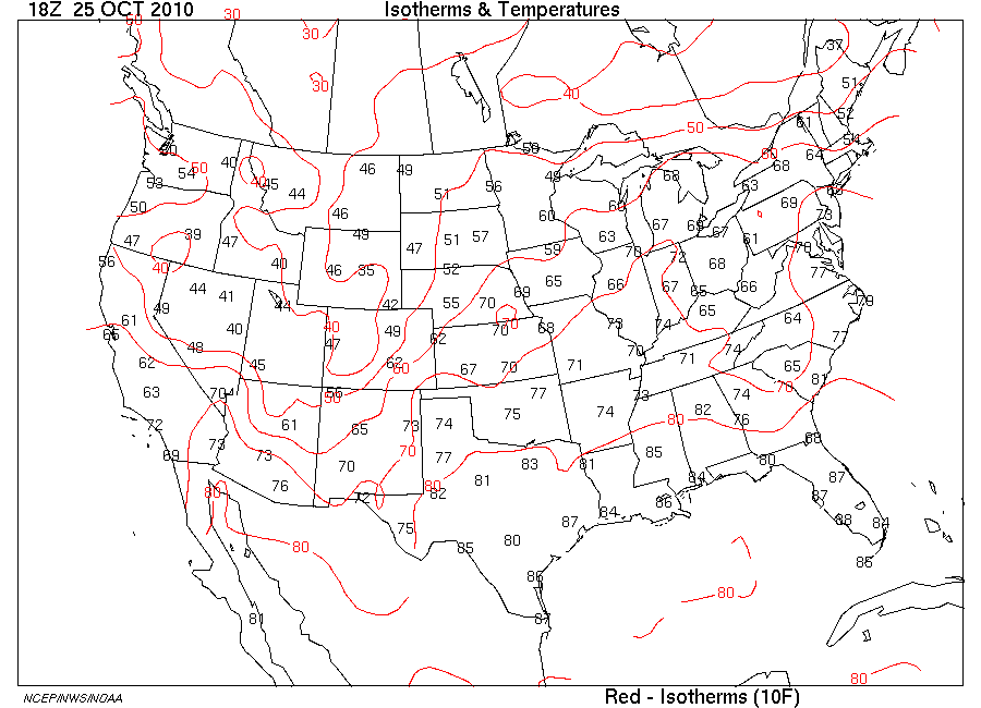
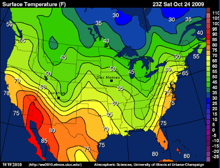
Isotherms are another example of where you are likely to encounter level curves. Isotherms are a plot in which the curves on the map connect locations that have the same temperature. A plot with lots of isotherms will allow you to see how the temperature changes over a region.
described in detail following the image
A map of the United States of America with numbers at locations of cities corresponding to temperatures. Red curves along the map connect points that have locations with constant values of temperature from 30 to 80 by steps of ten.
Figure 11.2.19. An isotherm map with temperatures at major cities (from NCEP/NWS/NOAA)


Activity 11.2.6.

In this activity, you will make contour plots by hand and look at how the spacing of contours in your plot should give an idea about how different surface shapes can be distinguished.
(a)
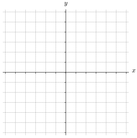
Let \(f(x,y) = x^2+y^2\text{.}\) Draw the level curves \(f(x,y) = k\) for \(k=1\text{,}\) \(k=2\text{,}\) \(k=3\text{,}\) and \(k=4\) on the axes below. Be sure to label the scale of the axes. Explain what the surface defined by \(f\) looks like.
described in detail following the image
A blank set of two dimensional axes with an unlabeled grid. The horizontal axis is labeled \(x\) and the vertical axis is labeled \(y\text{.}\)
(b)
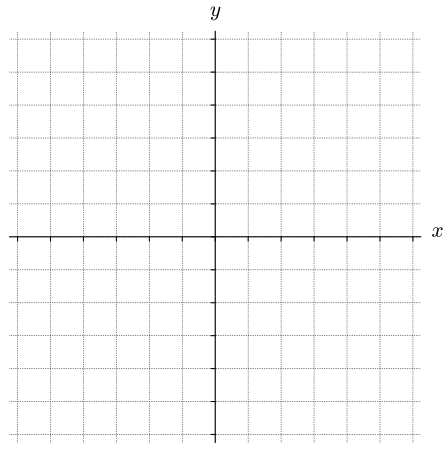
Let \(g(x,y) = \sqrt{x^2+y^2}\text{.}\) Draw the level curves \(g(x,y) = k\) for \(k=1\text{,}\) \(k=2\text{,}\) \(k=3\text{,}\) and \(k=4\) on the axes below. Use the same scale on these axes as in the previous part. Explain what the surface defined by \(g\) looks like.
described in detail following the image
A blank set of two dimensional axes with an unlabeled grid. The horizontal axis is labeled \(x\) and the vertical axis is labeled \(y\text{.}\)
(c)
Compare and contrast the graphs of \(f\) and \(g\text{.}\) How are they alike? How are they different? Use traces for each function to help answer these questions.
The traces and level curves of a function of two variables are curves in space. Traces are easier to parameterize as a curve in space because one input variable is fixed and the other input variable can act as the parameter. For example, the trace with \(y=b\) of the surface given by \(z=f(x,y)\) will be parameterized by \(\vr(t)=\langle t,b,f(t,b)\rangle\) because the \(z\)-coordinate can be expressed in terms of the fixed input value and the other input variable (as the parameter). Parameterizing contours, however, can be difficult and often relies on knowing the particular shape of the contours. Remember that it may not be possible to express a curve of the form \(k=f(x,y)\) with one coordinate as a function of the other.

Subsection 11.2.6 A gallery of functions

We end this section by considering a collection of functions and illustrating their surface graphs and contour plots. Many (but not all) of these surfaces will be familiar to you from SectionΒ 9.8, so now you will have an opportunity to see how the contour plots relate to the analyses you did in that section.
An interactive set of plots that consists of a three dimensional plot and a two dimensional plot. A drop down list at the top of the plots allows the user to select from Surface 1 to Surface 7. For Surface 1, the three dimensional plot shows a circular paraboloid opening toward the axis labeled \(z\) and the two dimensional plot shows a collection of concentric circles with rainbow colors that are labeled from 1 to 7 and spaced closer together as the circle’s radius increases. For Surface 2, the three dimensional plot shows top half of a cone opening toward the axis labeled \(z\) and the two dimensional plot shows a collection of concentric circles with rainbow colors that are labeled from .4 to 2.4 and equally spaced as the circle’s radius increases. For Surface 3, the three dimensional plot shows a circular paraboloid downward or away from the axis labeled \(z\) and the two dimensional plot shows a collection of concentric circles with rainbow colors that are labeled from 0 to -6 and spaced closer together as the circle’s radius increases. For Surface 4, the three dimensional plot shows a hyperbolic paraboloid or saddle surface and the two dimensional plot shows a collection of concentric hyperbolas with rainbow colors that are labeled from -.5 to 1.5 and spaced closer together as the hyperbolas appear farther from the origin. The hyperbolas oriented vertically are labeled with negative values and the hyperbolas oriented horizontally are labeled with positive values. For Surface 5, the three dimensional plot shows a curved surface that has a sinusoidal shape in the directions labeled \(x\) and \(y\text{.}\) The two dimensional plot shows a tilted grid of closed curves that alternate between positive and negative labels going from -1.5 to 1.5. For Surface 6, the three dimensional plot shows a curved surface that increases with a cubic shape along constant values of \(y\) and are parabolic facing up for constant values of \(x\text{.}\) The two dimensional plot shows a collection of curves around the point (-0.5,0) with labeled increasing from 0 to 8 as curves move away from the center of the figure. For Surface 7, the three dimensional plot shows a curved surface that consists of a single hill above the quadrants with both \(x\) and \(y\) positive or negative. The curved surface has depressions where \(x\) and \(y\) have different signs. The two dimensional plot shows a collection of concentric curves in each quadrant with the curves in the first and third quadrants labeled from 0 to 1.2 and the curves in the second and fourth quadrants labeled from 0 to -1.2.
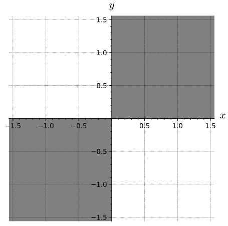
Figure 11.2.20. A plot of various functions and their contour plots

Exercises 11.2.7 Exercises

1.

Evaluate the function at the specified points.
\(f(x,y) = x+yx^{2}, \left(1,-2\right), \left(1,2\right), \left(-1,3\right)\)
At \(\left(1,-2\right)\text{:}\)
At \(\left(1,2\right)\text{:}\)
At \(\left(-1,3\right)\text{:}\)

2.

Suppose \(f(x,y)=\left(x^{2}-y^{2},2xy,x^{3}\right)\text{.}\) Compute the following values:
\(f(-2,5)\) \(=\)
\(f(5,-2)\) \(=\)
\(f(0,6)\) \(=\)
\(f(t^2,-2t)\) \(=\)
\(f(s+t,s-t)\) \(=\)

3.

Suppose \(f(x,y)=xy^{2}-1\text{.}\) Compute the following values:
\(f(0,-1)\) \(=\)
\(f(-1,0)\) \(=\)
\(f(0,0)\) \(=\)
\(f(-2,-1)\) \(=\)
\(f(t,6t)\) \(=\)
\(f(uv,u-v)\) \(=\)

5.

Evaluate the function at the specified points.
\(f(x,y) = y+xy^{4}, \left(-3,-1\right), \left(-2,1\right), \left(-5,-5\right)\)
At \(\left(-3,-1\right)\text{:}\)
At \(\left(-2,1\right)\text{:}\)
At \(\left(-5,-5\right)\text{:}\)

6.

The domain of the function \(f(x,y) = \sqrt x + \sqrt y\) is

11.

The balance, \(B\text{,}\) in dollars, in a bank account depends on the amount deposited, \(A\) dollars, the annual interest rate, \(r\) %, and the time, \(t\text{,}\) in months since the deposit, so \(B=f(A,r,t)\text{.}\)
(a) Is \(f\) an increasing or decreasing function of:
\(A\text{?}\)
\(r\text{?}\)
\(t\text{?}\)
(b) Interpret the statement \(f(1250, 3.25, 32) \approx 2974\) by writing a sentence, including units. Then use your sentence to complete the following:
The units of 1250 are:
The units of 3.25 are:
The units of 32 are:
The units of 2974 are:
.
(Note because this is all multiple choice, you will not see which parts of the problem are correct.)

13.

Match the surfaces with the verbal description of the level curves by placing the letter of the verbal description to the left of the number of the surface.
  1. \(\displaystyle z = \sqrt{(x^2 + y^2)}\)
  2. \(\displaystyle z = xy\)
  3. \(\displaystyle z = \sqrt{(25 - x^2 - y^2)}\)
  4. \(\displaystyle z = x^2 + y^2\)
  5. \(\displaystyle z = 2x + 3y\)
  6. \(\displaystyle z = 2x^2 + 3y^2\)
  7. \(\displaystyle z = \frac{1}{x-1}\)
  1. two straight lines and a collection of hyperbolas
  2. a collection of equally spaced concentric circles
  3. a collection of unequally spaced parallel lines
  4. a collection of equally spaced parallel lines
  5. a collection of concentric ellipses
  6. a collection of unequally spaced concentric circles

14.

For each surface, decide whether it could be a bowl, a plate, or neither. Consider a plate to be any fairly flat surface and a bowl to be anything that could hold water, assuming the positive z-axis is up.
  1. \(\displaystyle z = 1 - x^2 - y^2\)
  2. \(\displaystyle z = x^2 + y^2\)
  3. \(\displaystyle z = - \sqrt{ 4 - x^2 - y^2 }\)
  4. \(\displaystyle z = 5\)
  5. \(\displaystyle x + y + z = 4\)

15.

Suppose \(z = f(x,y) = \left(x^{2}+4\right)\sin\mathopen{}\left(y\right)+xy^{2}\text{.}\) By setting one variable equal to a constant (either \(x = c, y = c,\) or \(z = c\)), answer the following questions.
The intersection of the graph of \(f\) with the plane
is a sine curve if \(c =\) .
The intersection of the graph of \(f\) with the plane
is a line if \(c =\) .
The intersection of the graph of \(f\) with the plane
is a parabola if \(c =\) .

16.

The temperature adjusted for wind-chill, \(w\text{,}\) is a temperature which tells you how cold it feels, as a result of the combination of wind and temperature [see wind-chill]. See the table below, which gives temperature adjusted for wind-chill, \(w\text{,}\) as a function of temperature \(T\) and wind speed \(s\text{.}\)
\(T=35\) \(T=30\) \(T=25\) \(T=20\) \(T=15\) \(T=10\) \(T=5\) \(T=0\)
\(s=5\) 31 25 19 13 7 1 -5 -11
\(s=10\) 27 21 15 9 3 -4 -10 -16
\(s=15\) 25 19 13 6 0 -7 -13 -19
\(s=20\) 24 17 11 4 -2 -9 -15 -22
\(s=25\) 23 16 9 3 -4 -11 -17 -24
Use this table to make tables of the temperature adjusted for wind-chill (\(w\)) as a function of temperature for wind speeds 15 and 25 mph:
\(s = 15\text{:}\)
independent variable = =
dependent variable = =
\(s = 25\text{:}\)
independent variable = =
dependent variable = =

17.

(a) Describe a possible graph of the temperature, T, on an east-west line through Durango, Colorado, if the origin is at Durango, the positive x-axis corresponds to east of Durango, and the vertical z-axis is the temperature. For negative x within a few hundred miles of the origin, the sign of \(T'(x)\) is
, while for positive x a few hundred miles from the origin, the sign of \(T'(x)\) is
. We estimate that \(T(0) =\)
degrees Fahrenheit.
(b) Describe a possible graph of the temperature, T, on a north-south line through Des Moines, Iowa, if the origin is at Des Moines, the positive y-axis corresponds to north of Des Moines, and the vertical z-axis is the temperature. For negative y within a few hundred miles of the origin, the sign of \(T'(y)\) is
, while for positive y a few hundred miles from the origin, the sign of \(T'(y)\) is
. We estimate that \(T(0) =\)
degrees Fahrenheit.

18.

Find an equation for the contour of \(f(x, y) = 2 x^2 y + 6 x + 15\) that goes through the point \((4, 2)\text{.}\)
Equation:

19.

Write the level surface \(2 = \frac{2x^{2}+5y}{z}\) as the graph of a function \(f(x,y).\)
\(f(x,y) =\)

20.

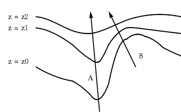
The figure below shows a contour map of a hill with two paths, \(A\) and \(B\text{.}\) The heights on the contours are \(z = z_0 = 100\text{,}\) \(z = z_1 = 175\text{,}\) and \(z = z_2 = 250\text{.}\)
(a) On which path, \(A\) or \(B\text{,}\) will you have to climb more steeply?
(b) On which path, \(A\) or \(B\text{,}\) will you probably have a better view of the surrounding countryside? (Assuming trees do not block your view.)
(c) Alongside which path is there more likely to be a stream?

21.

On a piece of paper, sketch each of the following surfaces:
(i) \(4 = x + 2 y + z\)
(ii) \(z = 4\)
Use your graphs to fill in the following descriptions of cross-sections of the surfaces.
(a) For (i) (\(4 = x + 2 y + z\)):
Cross sections with \(x\) fixed give
Cross sections with \(y\) fixed give
Cross sections with \(z\) fixed give
(b) For (ii) (\(z = 4\)):
Cross sections with \(x\) fixed give
Cross sections with \(y\) fixed give
Cross sections with \(z\) fixed give

22.

A car rental company charges a one-time application fee of 30 dollars, 60 dollars per day, and 11 cents per mile for its cars.
(a) Write a formula for the cost, \(C\text{,}\) of renting a car as a function of the number of days, \(d\text{,}\) and the number of miles driven, \(m\text{.}\)
\(C =\)
(b) If \(C = f(d, m)\text{,}\) then \(f(5, 530) =\)

23.

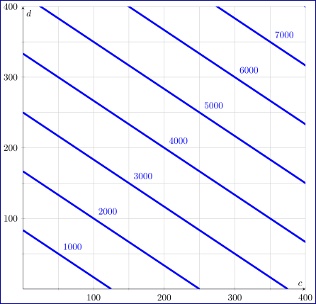
A store sells CDs at one price and DVDs at another price. The figure below shows the revenue (in dollars) of the music store as a function of the number, \(c\text{,}\) of CDs and the number, \(d\text{,}\) of DVDs that it sells. The values of the revenue are shown on each line.
$alt_text
(Hint: for this problem there are many possible ways to estimate the requisite values; you should be able to find information from the figure that allows you to give an answer that is essentially exact.)
  1. What is the price of a CD? dollars
  2. What is the price of a DVD? dollars

24.

Consider the concentration, C, (in mg/liter) of a drug in the blood as a function of the amount of drug given, x, and the time since injection, t. For \(0 \leq x \leq 6\) mg and \(t \geq 0\) hours, we have
\begin{equation*} C = f(x,t) = 20te^{-\left(6-x\right)t} \end{equation*}
\(f(1,2) =\)
Give a practical interpretation of your answer: \(f(1, 2)\) is
  • the amount of a 2 mg dose in the blood 1 hours after injection.
  • the concentration of a 1 mg dose in the blood 2 hours after injection.
  • the change in concentration of a 1 mg dose in the blood 2 hours after injection.
  • the amount of a 1 mg dose in the blood 2 hours after injection.
  • the change in concentration of a 2 mg dose in the blood 1 hours after injection.
  • the concentration of a 2 mg dose in the blood 1 hours after injection.

25.

A manufacturer sells aardvark masks at a price of $270 per mask and butterfly masks at a price of $520 per mask. A quantity of a aardvark masks and b butterfly masks is sold at a total cost of $600 to the manufacturer.
(a) Express the manufacturer’s profit, P, as a function of a and b.
\(P(a,b) =\) dollars.
(b) The curves of constant profit in the ab-plane are

26.

Consider the concentration, \(C\text{,}\) in mg per liter (L), of a drug in the blood as a function of \(x\text{,}\) the amount, in mg, of the drug given and \(t\text{,}\) the time in hours since the injection. For \(0 \leq x \leq 4\) and \(t \geq 0\text{,}\) we have \(C = f(x,t) = t e^{-t(5-x)}\text{.}\)
Graph the following two single variable functions on a separate page, being sure that you can explain their significance in terms of drug concentration.
(a) \(f(4,t)\)
(b) \(f(x,2.5)\)
Using your graph in (a), where is \(f(4,t)\)
a maximum? \(t =\)
a minimum? \(t =\)
Using your graph in (b), where is \(f(x,2.5)\)
a maximum? \(x =\)
a minimum? \(x =\)

27.

By setting one variable constant, find a plane that intersects the graph of \(z = 2y^{2}-4x^{2}+2\) in a:
(a) Parabola opening upward: the plane =
(Give your answer by specifying the variable in the first answer blank and a value for it in the second.)
(b) Parabola opening downward: the plane =
(Give your answer by specifying the variable in the first answer blank and a value for it in the second.)
(c) Pair of intersecting straight lines: the plane =
(Give your answer by specifying the variable in the first answer blank and a value for it in the second.)

28.

The Ideal Gas Law, \(PV = RT\text{,}\) relates the pressure (\(P\text{,}\) in pascals), temperature (\(T\text{,}\) in Kelvin), and volume (\(V\text{,}\) in cubic meters) of 1 mole of a gas (\(R = 8.314 \ \frac{\text{J} }{\text{ mol } \ \text{K} }\) is the universal gas constant), and describes the behavior of gases that do not liquefy easily, such as oxygen and hydrogen. We can solve the ideal gas law for the volume and hence treat the volume as a function of the pressure and temperature:
\begin{equation*} V(P,T) = \frac{8.314T}{P}. \end{equation*}

(a)

Explain in detail what the trace of \(V\) with \(P=1000\) tells us about a key relationship between two quantities.

(b)

Explain in detail what the trace of \(V\) with \(T=5\) tells us.

(c)

Explain in detail what the level curve \(V = 0.5\) tells us.

(d)

Use 2 or three additional traces in each direction to make a rough sketch of the surface over the domain of \(V\) where \(P\) and \(T\) are each nonnegative. Write at least one sentence that describes the way the surface looks.

(e)

Based on all your work above, write a couple of sentences that describe the effects that temperature and pressure have on volume.

29.

When people buy a large ticket item like a car or a house, they often take out a loan to make the purchase. The loan is paid back in monthly installments until the entire amount of the loan, plus interest, is paid. The monthly payment that the borrower has to make depends on the amount \(P\) of money borrowed (called the principal), the duration \(t\) of the loan in years, and the interest rate \(r\text{.}\) For example, if we borrow $18,000 to buy a car, the monthly payment \(M\) that we need to make to pay off the loan is given by the formula
\begin{equation*} M(r,t) = \frac{1500r}{1-\frac{1}{\left(1+\frac{r}{12}\right)^{12t}}}. \end{equation*}

(a)

Find the monthly payments on this loan if the interest rate is 6% and the duration of the loan is 5 years.

(b)

Create a table of values that illustrates the trace of \(M\) with \(r\) fixed at 5%. Use yearly values of \(t\) from 2 to 6. Round payments to the nearest penny. Explain in detail in words what this trace tells us about \(M\text{.}\)

(c)

Create a table of values that illustrates the trace of \(M\) with \(t\) fixed at 3 years. Use rates from 3% to 11% in increments of 2%. Round payments to the nearest penny. Explain in detail what this trace tells us about \(M\text{.}\)

(d)

Consider the combinations of interest rates and durations of loans that result in a monthly payment of $200. Solve the equation \(M(r,t) = 200\) for \(t\) to write the duration of the loan in terms of the interest rate. Graph this level curve and explain as best you can the relationship between \(t\) and \(r\text{.}\)

30.

Consider the function \(h\) defined by \(h(x,y) = 8 - \sqrt{4 - x^2 - y^2}\text{.}\)

(a)

What is the domain of \(h\text{?}\) (Hint: describe a set of ordered pairs in the plane by explaining their relationship relative to a key circle.)

(b)

The range of a function is the set of all outputs the function generates. Given that the range of the square root function \(g(t) = \sqrt{t}\) is the set of all nonnegative real numbers, what do you think is the range of \(h\text{?}\) Why?

(c)

Choose 4 different values from the range of \(h\) and plot the corresponding level curves in the plane. What is the shape of a typical level curve?

(d)

Choose 5 different values of \(x\) (including at least one negative value and zero), and sketch the corresponding traces of the function \(h\text{.}\)

(e)

Choose 5 different values of \(y\) (including at least one negative value and zero), and sketch the corresponding traces of the function \(h\text{.}\)

(f)

Sketch an overall picture of the surface generated by \(h\) and write at least one sentence to describe how the surface appears visually. Does the surface remind you of a familiar physical structure in nature?