In the previous sections, we introduced vector-valued functions, which provided us with a useful tool for thinking about curves in three-dimensional space. We have also seen how the calculus operations of limits, derivatives, and integrals apply to these functions. In single-variable calculus, you likely learned that displacement (net change in position) and total distance traveled for an object moving in one-dimension will not be the same if the object changes direction. For motion along a curve in two or more dimensions, we have a similar distinction. For instance, consider the curve in Figure 10.3.1.
An oriented curve from a point \(P\) to a point \(Q\text{.}\) The curve moves up and left from the point \(P\text{,}\) then turns up and to the right before moving down and right to the point \(Q\text{.}\)
However, if this curve is a portion of a road on which we drive a car, the distance traveled as measured by the change in the car’s odometer value from point \(P\) to point \(Q\) will be different than the straight-line distance \(\vert PQ\vert\) calculated by the distance formula. You likely saw how to calculate the length of a portion of a curve \(y=f(x)\) in your single-variable calculus class. In this section, we will use the idea of vector-valued functions to find the lengths of a larger family of curves.
In Preview Activity 10.1.1 and Preview Activity 10.2.1 we saw how the position reported by the location tracking system (LTS) of a self-driving car corresponds to a vector-valued function that describes the location of the car at a given time. We want to relate the location at different times to properties about how the car is being driven. In order to attract investors and drive shareholder value in Steer Clear, you decide to use the location tracking system’s output to build a customized navigation and telemetry tool for a self-driving car. The first element you will need to build is a way to use the LTS output to calculate how far the car has driven in a given time.
In your testing center (an abandoned parking garage), you drive your car up a ramp and note that the LTS recorded that the car had coordinates of \(\langle 10,-5,0\rangle\) at \(t=0\) and \(\langle -8,10,12\rangle\) at \(t=30\) seconds. The units on each component of the coordinate vectors are meters. What is the distance between initial (\(t=0\)) and final (\(t=30\)) positions of the car? This is the displacement of your total trip.
Do you think the distance the car actually traveled is greater than, less than, or exactly the same as your answer to part a? Write a couple of sentences to explain your reasoning.
In order to get more information for your telemetry system, you decide to pull the location data from your drive up the parking ramp every 10 seconds. The LTS gives the following data:
Do you think your estimate from part c is greater than, less than, or equal to the actual distance traveled? Write a couple of sentences to explain your reasoning.
You look into the documentation on your location tracking system and see that you can specify how often the software will output location data. You decide that getting the location every half second seems like a good idea. How many data points will that correspond to for your drive up the ramp? Write a couple of sentences to describe what steps you would take with this new location data to calculate a better estimate on the distance traveled by your car. How might you go about finding the exact distance traveled by your car?
The central question we want to answer in this section is “Given a curve \(C\) from \(P\) to \(Q\text{,}\) what is the length of \(C\text{?}\)” We will be able to answer this question for well-behaved curves by applying the classic calculus approach to the ideas you investigated in the Preview Activity. To do this, we approximate the length of the curve \(C\) by computing the length of line segments between points on \(C\text{.}\) We will call these intermediate points \(\vr_0,\vr_1,...,\vr_n\text{.}\) Remember that we are specifying location using vectors graphed in standard position. Using vectors to specify position means that the corresponding line segments between successive positions can be represented by the vector difference \(\Delta\vr_i = \vr_{i}-\vr_{i-1}\text{.}\)
An oriented curve from a point \(P\) to a point \(Q\text{.}\) Point \(P\) is labeled as \(\vr_0\) and point \(Q\) is labeled as \(\vr_n\text{.}\) There are five intermediate points drawn as well as vectors connecting consecutive intermediate points. The vector from \(\vr_{3}\) to \(\vr_4\) is labeled \(\Delta\vr_4 = \vr_4-\vr_{3}\text{.}\)
This leads to an approximation for the length of \(C\) given by the sum of the lengths of the vectors \(\Delta\vr_i = \vr_i-\vr_{i-1}\text{.}\) Using \(\Delta x_i\text{,}\)\(\Delta y_i\text{,}\) and \(\Delta z_i\) to denote the change in each component, the magnitude of \(\Delta \vr_i\) is determined by the distance formula as we saw in the previous chapter:
Use the slider on Figure 10.3.3 to change the number of segments used in the approximation of the arc length of \(C\text{.}\) Notice that as the number of segments increases, the difference between the actual length of the curve and the line segments gets smaller. You can also see how the sum of the lengths of the blue segments will approach the true length of the curve, which is approximately \(6.3286\text{.}\)
An interactive two dimensional plot with an oriented curve from a point \(P\) to a point \(Q\text{.}\) The curve moves up and left from the point \(P\text{,}\) then turns up and to the right before moving down and right to the point \(Q\text{.}\) The slider above the plot changes the number of line segments drawn between intermediate points on the oriented curve. Line segments are drawn in blue between intermediate points on the curve. The length of the blue line segments is displayed as an approximation to the true arc length of the oriented curve.
Notice that the approximation above does not involve a parameterization of \(C\text{.}\) In general, it is easiest to generate the positions \(\vr_i\) by evaluating a parameterization at different \(t\)-values. We will use \(\vr(t)=\langle x(t),y(t),z(t)\rangle\) as a parameterization of \(C\) to specify points between \(P\) and \(Q\text{.}\)
Specifically, if \(\vr(t)\) is a parameterization of \(C\) with \(P=\vr(a)\) and \(Q=\vr(b)\text{,}\) we can divide \(C\) into \(n\) parts given by \(\vr_i=\vr(t_i)\) where \(t_i=a+ i \Delta t\) with \(\Delta t= \frac{b-a}{n}\text{.}\) This divides \(C\) into parts that correspond to equal steps in the parameter \(t\text{.}\) (Note that these parts will, in general, not correspond to parts with equal length.)
This process leads to an approximation used in the first step of the classic calculus approach. Since this approximation approaches the actual length as we use smaller and smaller steps, we define the arc length as follows:
Since we want to shrink the step size \(\Delta t\) to get better approximations, we now rewrite the approximation to allow us to see how the approximation changes as we consider smaller values of \(\Delta t\text{.}\) To do this, note that assuming \(x(t)\) is differentiable, since \(x'(t_i)\approx \Delta x_i/\Delta t\text{,}\) we can write that \(\Delta x_i\approx x'(t_i)\Delta t\text{.}\) This applies equally well for both \(y\) and \(z\text{,}\) so this leads us to
This refines the approximation and completes the second step in the classic calculus approach. Now we have set up the approximation as a Riemann sum. In particular, this approximation is a Riemann sum of the function \(\sqrt{\left(x'(t_i)\right)^2 + \left(y'(t_i)\right)^2 + \left(z'(t_i)\right)^2}\) which will simplify as \(\Delta t\) goes to 0. Thus the limit of the Riemann sum from the definition of arc length gives a definite integral
If \(\vr(t)\) parameterizes a curve \(C\) on an interval \([a,b]\) for which \(\vr\, '(t)\) exists at each point, then the length\(L\) of \(C\text{,}\) is given by
\begin{equation}
L = \int_a^b \vecmag{\vr\, '(t)} \, dt.\tag{10.3.1}
\end{equation}
Note that formula (10.3.1) applies to curves in any dimensional space. Moreover, this formula has a natural interpretation: If \(\vr(t)\) records the position of a moving object, then \(\vr\, '(t)=\vv(t)\) is the object’s velocity and \(\vecmag{\vr\, '(t)}\) its speed. Formula (10.3.1) says that we can integrate the speed of an object traveling over the curve to find the distance traveled by the object. Thinking in terms of units, if we are measuring distance in meters and time in seconds, the units on \(\vecmag{\vr\, '(t)}\) will be meters per second and the units on \(dt\) will be seconds. Thus, the units on the integral will be meters, which is exactly what we expect when finding the length of a curve or distance traveled by an object along a curve. This formula is analogous to the formula for finding the arc length of a graph from single-variable calculus.
Use your parameterization from the previous part in the definite integral of Theorem 10.3.5 to calculate the circumference of a circle of radius \(3\text{.}\)
Notice here that while we focused on the circle of radius \(3\text{,}\) changing to the more general radius of \(R\) for the circle gives a parameterization of \(\langle R\cos(t),R\sin(t)\rangle\) with \(0\leq t\leq 2\pi\text{.}\) The work to use the arc length integral to find the circumference of this circle requires only small modifications to the work you did in this activity.
Exercise 7 will apply Definition 10.3.4 and Theorem 10.3.5 to arrive at a formula for the length of a graph given by \(y=f(x)\) that may be familiar from single-variable calculus courses.
In Activity 10.3.2, we considered parameterizations of a circle and a helix. The computation of the arc length in these problems was made easier by the fact that the speed of an object with motion described by the parameterizations used did not depend on the time \(t\text{.}\) That is, the speed of an object moving according to the parameterization was constant. Moving with constant speed is always feasible. For example, we can set our self-driving car to move at a constant speed of 60 miles per hour, and the car then moves with constant speed. (Of course, this is probably only recommended on a road where no obstacles or other vehicles will appear.) However, finding a parameterization with constant speed may involve some complex algebra, as we will see while working through this section.
We will focus on finding a parameterization with unit speed. That is, one for which \(\vecmag{\vv(t)} = \vecmag{\vr\, '(t)} = 1\) for all values of \(t\text{.}\) We call such a parameterization a unit speed parameterization of the curve. The key idea involves recognizing that, in general, distance along the curve is not the same as the parameter being used. If an object moves with constant speed one, then the numerical value of the distance it travels is the numerical value of the time elapsed. For example, if you walk at exactly 1 meter per second for 47 seconds, how far have you gone? If you walk at exactly 1 meter per second, how long will it take you to travel 47 meters? The answer to both is 47 but the units are different. Remember that we do not have to walk in a straight line (i.e., with constant direction) to keep speed constant.
As a more concrete illustration of this idea, consider the curve defined by the parabola \(y = x^2/2\) with \(x\in[0,2]\text{.}\) We can parameterize this curve by \(\vr(t) = \langle t, t^2/2\rangle\) for \(t\in[0,2]\text{.}\)Figure 10.3.6 shows a plot of this parabola with equally-spaced points in the parameter \(t\) on the left. You can see in the plot on the left that equally-spaced points based on parameter values are not separated by equal distances along the curve. On the right, however, the points are equally-spaced by arc length. By this we mean that the distance along the curve between the point labeled \(s=0.5\) and the point labeled \(s=1.0\) is \(0.5\text{.}\) Similarly, the distance along the curve between the point labeled \(s=0.5\) and the point labeled \(s=2.5\) is \(2\text{.}\) For this reason, a unit speed parameterization is also often called a parameterization by arc length.
A two dimensional plot with the coordinates between 0 and 2. A parabola opening toward the top of the plot is shown in blue with vertex at the origin and going through the point \((2,2)\text{.}\) Intermediate points are shown for \(t=0,0.5,1,1.5,2\) on the left and are not equally spaced on the curve. Equally spaced intermediate points are shown on the right and are labeled \(s=0,0.5,1,,1.5,2,2.5\text{.}\)
In many ways, a parameterization with unit speed is a natural parametrization. Consider an interstate highway cutting across a state. One way to parametrize the curve defined by the highway is to drive along the highway and record our position at every time \(t\text{,}\) thus creating a function \(\vr(t)\text{.}\) If we encounter an accident or road construction, however, this parametrization might not be at all relevant to another person driving the same highway. A parameterization using unit speed is like using the mile markers on the side of the road to specify our position on the highway. If we know how far we’ve traveled along the highway, we know exactly where we are. Another way to think about this is that by driving at exactly one mile per hour, we can put mile markers down every hour.
In this example, we look at a linear path and explore how to write a parameterization that moves with unit speed. We will look at the parameterization of the line through \((1,2,3)\) and \((2,0,5)\text{.}\) We are using these values to make the calculations less abstract but there is nothing special about these values and the methods will work for any linear parameterization.
An easy-to-find parameterization will have the base point \((1,2,3)\) and direction vector given by the difference between our points, \(\langle 2-1, 0-2, 5-3\rangle = \langle 1,-2,2 \rangle\text{.}\) This leads to an initial parameterization of the line as \(\vr(t)=\langle 1,2,3\rangle + t \langle 1,-2,2 \rangle\text{.}\) Notice that with this parameterization, restricting to \(0\leq t\leq 1\) gives a domain for \(\vr(t)\) for the line segment from \((1,2,3)\) when \(t=0\) to \((2,0,5)\) when \(t=1\text{.}\) The arc length of this segment can be computed using the distance formula, so it is \(3\text{.}\)
We want to convert this to a parameterization with unit speed. To think of this another way, we are aiming to have the parameter value when we reach the point \((2,0,5)\) be equal to the distance from the base point \((1,2,3)\text{.}\) This will mean we seek a parameterization \(\vr_1(s)\) where the domain \(0\leq s\leq 3\) corresponds to the line segment from \((1,2,3)\) to \((2,0,5)\text{.}\) The speed of this parameterization is
This means that we need to adjust our parameterization to travel \(3\) times slower, which can be accomplished by replacing \(t\) in our parameterization with \(s=t/3\text{.}\) In other words, we adjusted the parameter used to make sure the speed with respect to the new parameter will be one. This adjustment was easy to do because the amount we needed to change the parameter did not change at different times.
Algebraically, we can describe this change by thinking of \(\vr(t)\) as the “old” parameterization with parameter \(t\text{,}\) and we aim to replace \(t\) with a function \(s(t)\) so that \(\vecmag{\vr_1\, '(s(t))}=1\) for all \(t\text{.}\) For this linear path, the choice of \(s(t) = t/3\) means that applying the chain rule to \(\vecmag{\vr_1\, '(s)}\) gives
The left part of equation (10.3.2) shows the important idea needed to find a unit speed parameterization: we can adjust the speed of the parameterization. This requires that we pick a transformation \(s(t)\) to satisfy
Algebraically, this is very difficult to write out in closed form. However, it will be possible because the arc length traveled as a function of the parameter cannot decrease. If we make a two-dimensional plot with the parameter value on the horizontal axis and the arc length traveled on the vertical axis, then we have a graph that passes the horizontal line test. This means that this function has an inverse! An example of this kind of plot is shown in Figure 10.3.8. The point highlighted on the graph indicates that at the parameter value \(t=4\text{,}\) the arc length from the point with \(t=0\) (or the distance traveled by an object following the curve from \(t=0\) to \(t=4\)) is approximately \(48.134\text{.}\) In other words, when finding a parameterization by arc length or unit speed parameterization, we will need to arrive at the same point on the curve when the parameter value is \(48.134\text{.}\)
Axes for the first quadrant. The horizontal axis is labeled with time \(t\) and the vertical axis is labeled arc length \(s\text{.}\) The graph depicts a function that starts at the origin and increases, although the rate of increase varies. There is also a point identified on the graph with \(t\)-coordinate \(4\) and \(s\)-coordinate approximately \(48\text{.}\) Dashed lines go from the axes to this point.
Figure10.3.8.A plot of the arc length traveled as a function of the parameter value to that point for \(\vr(t)=\langle 3t\cos(4t)\sin(3-2t),t-\cos(2+t)\rangle\)
for \(t \geq 0\text{.}\) Our goal is to find a unit speed parameterization of \(C\text{.}\) The first step is to find the speed of our current parameterization:
An important element of this example is that our speed is not constant but still algebraically easy enough to work with for later calculations. Note that because we have stated that \(t \geq 0\) we only need to consider the positive square root calculation.
Next, we will calculate \(s(a)\text{,}\) the arc length traveled from \(t=0\) to \(t=a\) along the curve \(C\) in order to help us figure out how to transform our parameterization into one with unit speed. We use Theorem 10.3.5 to compute the arc length of \(C\) as \(t\) goes from \(0\) to \(a\text{.}\)
This computation shows us that the arc length traveled from \(t=0\) to \(t=a\) along the curve \(C\) is \(a^2+4a\text{.}\) Remember that we want to transform our parameterization to have unit speed, which will mean that the arc length up to a point and the parameter value corresponding to that point will be the same value. We want to state a function that has an input of arc length along the curve \(C\) and outputs the time at which the original parameter reaches that location. In other words, we want the inverse function of \(s(a)=a^2+4a\text{,}\) because the output of \(s(a)\) is arc length up to the point corresponding to the parameter value \(a\text{.}\) In Figure 10.3.10, we show the graph of the function \(s(a)\text{.}\)
The graph of an increasing curve in the first quadrant. The horizontal axis is labeled \(t\) and the vertical axis is labeled \(s\text{.}\) A point on the graph is identified and labeled \((a,s(a))\text{.}\) Vertical and horizontal dashed lines from this point to the axes are included as well.
Since \(a \geq 0\text{,}\) we can solve the equation \(s = a^2+4a\) (or \(a^2+4a-s=0\)) for \(a\) to obtain \(a(s) = \frac{-4 +\sqrt{16+4s}}{2} = -2 + \sqrt{4+s}\text{.}\) Note again that by restricting to positive parameter values, we only need to consider one solution. Another way of thinking about this is that the point labeled \((a,a^2+4a)\) in Figure 10.3.10 could also be labeled \((-2+\sqrt{4+s},s)\text{.}\)
Let’s take a moment to further discuss the relationship between our two functions and their composition. The original parameterization \(\vr(t)\) has inputs of parameter values (\(t\)) and outputs corresponding to locations on our curve \(C\text{.}\) The function value \(s(a)\) gives the arc length along \(C\) from \(t=0\) to \(t=a\text{,}\) so the inputs to this function are parameter values and the outputs are arc lengths. The new function \(a(s)\) is the inverse of \(s\text{,}\) and thus its input is arc length. (Specifically, the input is the arc length traveled from \(t=0\) to \(t=a\) along the curve \(C\text{.}\)) The output from \(a(s)\) is a parameter value of the original parameterization corresponding to when the arc length is \(s\text{.}\)
We can now compose our result of \(a=-2+\sqrt{4+s}\) with the original parameterization to get our unit speed parameterization. Specifically, we claim that \(\vr(a(s))\) will be a unit speed parameterization. Remember that a unit speed parameterization of a curve is equivalent to the idea that “parameter value = time elapsed = arc length traveled”.
The parameterization \(\vr(a(s))\) is a unit speed parameterization because the parameter \(s\)is the amount of arc length traveled. In terms of the mile marker analogy, the value of \(s\) is the value you see on the mile marker. The input of the composition \(\vr(a(s))\) will be the arc length traveled. The “inner” function, \(a(s)\text{,}\) outputs the parameter value of the original parameterization where that arc length is achieved. (Keep in mind Figure 10.3.10, which illustrates the inverse relationship between \(a\) and \(s\text{.}\)) This means that \(\vr(a(s))\) outputs the location on \(C\) where an arc length of \(s\) is achieved.
To illustrate the concepts of the previous paragraph concretely, we return to the algebra of our problem. For our example, the composition \(\vr(a(s))\) gives the following as the unit speed parameterization:
The crucial step, both algebraically and conceptually, in our work was the inverse function of \(s(a)\text{,}\) which was relatively simple for this example. In general, this can be difficult to write out explicitly.
These examples illustrate a general method for finding a unit speed parameterization. Evaluating an arc length integral and finding the formula for the inverse of a function can each be difficult. Although this process is always theoretically possible, it is frequently not practical to parameterize a curve in terms of arc length. However, we can guarantee that such a parameterization exists, and this observation plays an important role in the next section.
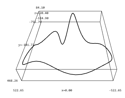
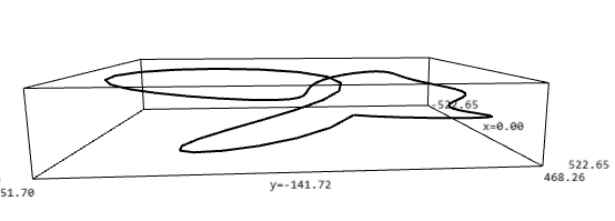
A plot of the a race track with a long straightaway, followed by a gentle curve, then several back and forth turns and another gentle turn from the side which shows how the racetrack changes elevation along the circuit.
All of the drivers are going the same way around the track, all start at the same location at \(t=0\text{,}\) all complete one lap of the track, and all of the cars have perfect grip of the road (the race cars are never sliding). The picture of the racetrack above is given so you have an example to help you think about the tasks in this problem, not because any particular feature of the track needs to be considered for the following activity.
Activity10.3.3.Is it a property of the driver or the road?
In this activity, we want to determine if the different measurements we have described are a property of the driver or the road. A measurement is a property of the driver provided that the values of that measurement can be different for different drivers when measured at the same location on the racetrack. A measurement is a property of the road provided that different drivers must have the same values when measured at the same location on the racetrack.
Remember that we are not asking if the driver or road can control time. We are asking if the elapsed time is the same for all drivers at a fixed point on the racetrack or if drivers can have a different elapsed time to a particular location on the racetrack.
You should make sure you understand that the measurements for different drivers must be made at the same location on the track, as stated above. Your explanation sentence may sound a little silly.
Now that we are warmed up, let’s look at some more interesting measurements. The car’s speedometer reading measures how fast (as a scalar) the car is moving. Is the car’s speedometer reading a property of the driver or the road? Be sure to explain your answer.
The racecar’s odometer measures the distance traveled by the car. Every car’s odometer is set to be zero at the start of the race. Is the car’s odometer reading a property of the driver or the road? Be sure to explain your answer.
When we are using the analogy of the racetrack for a curve in space, each different driver corresponds to a different parameterization of the curve. If a measurement is a property of the driver, that measurement can take different values for different parameterizations. If a measurement is a property of the road, then every parameterization must have the same measured value when considered at the same location on the curve. In short, parameterizations are drivers and the curve in space is the racetrack.
A parameterization with unit speed is useful because when we move with unit speed, the parameter value is equal to the arc length traveled to that point.
The WeBWorK problems are written by many different authors. Some authors use parentheses when writing vectors, e.g., \((x(t),y(t),z(t))\) instead of angle brackets \(\langle x(t),y(t),z(t) \rangle\text{.}\) Please keep this in mind when working WeBWorK exercises.
Let \(y = f(x)\) define a smooth curve in 2-space. Parameterize this curve and use Equation (10.3.1) to show that the length of the curve defined by \(f\) on an interval \([a,b]\) is
In this exercise, we will make the unit speed parameterization for the curve parameterized by \(\vr(t)=\langle \frac{3}{2} t^2,2t^2,\frac{5}{3}t^3\rangle\) for \(t\in[0,a]\text{.}\)
Calculate the speed for the parameterization \(\vr(t)=\langle \frac{3}{2} t^2,2t^2,\frac{5}{3}t^3\rangle\text{.}\) Factor out as large a power of \(t\) out of the square root as possible.
Use your speed calculation from above to compute the arc length on our curve \(C\) as \(t\) goes from 0 to \(a\text{.}\) Your answer should be in terms of \(a\text{.}\)
Your previous step should have created a function \(s(a)\) which outputs the arclength traveled on \(C\) for \(t\) from 0 to \(a\text{.}\) Find the inverse function, \(a(s)\text{,}\) that outputs the time past 0 that is needed to travel \(s\) along the curve.