Print preview

Section 12.4 Double Integrals over General Regions

Motivating Questions

How do we define a double integral over a non-rectangular region?
What general forms do iterated integrals over non-rectangular regions have?

Notes to the Instructor and Dependencies.

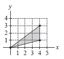
This section builds off of the previous two sections and generalizes the horizontal or vertical slicing of the region of integration and demonstrates how this geometric description exactly matches with the algebraic description given by an iterated integral. There are several important conceptual checks that you should pay attention to:

identification of horizontally or vertically simple regions,
understanding when double integrals will be positive/negative/zero without any calculations (Activity 12.4.2), and
identifying when the algebra of an iterated integral does not make sense as a double integral (Activity 12.4.4).

There is a lot for students to practice in this section, so we recommend spending a couple of class periods on this topic. Spending 50 minutes on writing the inequalities that describe a region as vertically simple or horizontally simple (doing the activities through Activity 12.4.4) is quite reasonable. These ideas will be used throughout every section for this chapter and through most of Chapter 13, so making sure students understand what a double integral measures and and how to set up appropriate iterated integrals is critical.

Subsection 12.4.1 Introduction

Recall from Section 12.2 that we defined the double integral of a continuous function \(f = f(x,y)\) to measure the volume of the region beneath the graph of \(f\) over a region of input points. If we consider the set of points in a rectangle \(R\) with \(a\leq x\leq b\) and \(c\leq y\leq d\text{,}\) then we can calculate the double integral using a Riemann sum

\begin{equation*} \iint_R f(x,y) \, dA = \lim_{m,n \to \infty} \sum_{j=1}^n \sum_{i=1}^m f(x_{ij}^*, y_{ij}^*) \cdot \Delta A\text{.} \end{equation*}

Furthermore, we have seen in Fubini’s Theorem that we can evaluate a double integral \(\displaystyle{\iint_R f(x,y) \, dA}\) over \(R\) as an iterated integral of either of the forms

\begin{equation*} \int_a^b \int_c^d f(x,y) \, dy \, dx \quad \quad \text{ or } \quad \quad \int_c^d \int_a^b f(x,y) \, dx \, dy. \end{equation*}

Most applied or theoretical problems involve regions of inputs that are not rectangles. Therefore, we want to extend the idea of using iterated integrals to allow us to evaluate double integrals over nonrectangular regions. We explore one such example in the following preview activity.

Preview Activity 12.4.1.

A tetrahedron is a three-dimensional figure with four faces, each of which is a triangle. A picture of the tetrahedron \(T\) with vertices \((0,0,0)\text{,}\) \((1,0,0)\text{,}\) \((0,1,0)\text{,}\) and \((0,0,1)\) is shown in Figure 12.4.1. By using techniques from Section 9.7, we can find that an equation for this plane is

\begin{equation*} z=1-(x+y)\text{.} \end{equation*}

However, we cannot directly use the methods we have developed so far involving double integrals to find the volume of a solid above the \(xy\)-plane and below a surface \(z=f(x,y)\text{,}\) as the base of the tetrahedron is not rectangular. This Preview Activity generalizes the work we have done so far with double integrals to understand how we can use a double integral to compute the volume of this tetrahedron. To do this, we will apply the Classic Calculus Approach.

Coordinate axes for \(xyz\)-space showing a solid region with vertices \((0,0,0)\text{,}\) \((1,0,0)\text{,}\) \((0,1,0)\text{,}\) and \((0,0,1)\text{.}\) Each face of the solid is a triangle.

Figure 12.4.1. The tetrahedron \(T\) with vertices \((0,0,0)\text{,}\) \((1,0,0)\text{,}\) \((0,1,0)\text{,}\) and \((0,0,1)\)

(a)

As our first step in applying the Classic Calculus Approach, we approximate the tetrahedron by using three triangular prisms with bases parallel to the \(yz\)-plane. Specifically, the bases lie in the planes \(x=0\text{,}\) \(x=1/3\text{,}\) and \(x=2/3\text{.}\) We show these three triangular prisms in Figure 12.4.2.

Coordinate axes for \(xyz\)-space showing three triangular prisms with triangular bases parallel to the \(yz\)-plane. The triangular cross sections that are the bases of the three prisms are located in the planes \(x=0\text{,}\) \(x=1/3\text{,}\) and \(x=2/3\text{.}\)

Figure 12.4.2. A decomposition of the tetrahedron into three triangular prisms with base parallel to the \(yz\)-plane

The volume of each triangular prism is the cross sectional area of the prism’s base times the thickness of the prism. Find the cross sectional area for the three prisms shown in the figure.

(b)

Write a sum in the form below that completes Step 1 of the Classic Calculus Approach.

\begin{equation*} \sum_{i=1}^3 (\text{cross sectional area})\cdot (\text{prism width}) \end{equation*}

(c)

For Step 2 of the Classic Calculus Approach, we generalize the approximation above to work for \(n\) triangular prisms of equal width. To do this, we must find the cross sectional area at an arbitrary location \(x=a\text{.}\) Create a carefully-labeled two-dimensional drawing of the highlighted cross section in Figure 12.4.3 that can be interpreted for any value of \(a\) where the plane \(x=a\) intersects the tetrahedron. Your drawing should be in the \(yz\)-plane, and you should label components of your diagram in terms of the parameter \(a\text{.}\) Make sure to write an equation for the line that forms the hypotenuse of the triangle, which should be expressed in terms of \(y\text{,}\) \(z\text{,}\) and \(a\text{.}\)

Coordinate axes for \(xyz\)-space showing a solid region with vertices \((0,0,0)\text{,}\) \((1,0,0)\text{,}\) \((0,1,0)\text{,}\) and \((0,0,1)\text{.}\) Each face of the solid is a triangle. There is also a triangular cross section highlighted. This cross section is parallel to the \(yz\)-plane. It is marked \(x=a\text{.}\)

Figure 12.4.3. The tetrahedron \(T\) with cross section along \(x=a\) shown

(d)

Write a \(dy\) integral for the area of the cross section you drew in the previous part. Your integral will include \(a\) in multiple ways. Verify that your integral gives the same value you found earlier for the \(a=1/3\) cross sectional area.

(e)

To complete Step 2 of the Classic Calculus Approach, we approximate the volume by a sum. Specifically, if we denote the cross sectional area of the \(i\)th triangular prism by \(\text{CSA}_i\text{,}\) then the volume is approximated by

\begin{equation*} \sum_{i=1}^n \text{CSA}_i\cdot \Delta x\text{.} \end{equation*}

By the Classic Calculus approach, the volume of the tetrahedron is

\begin{equation} \lim_{n\to\infty}\sum_{i=1}^n \text{CSA}_i\cdot \Delta x = \int_0^1 \text{CSA(x)}\, dx\text{,}\tag{12.4.1} \end{equation}

where \(\text{CSA}(x)\) denotes the cross sectional area for position \(x\text{.}\)

In the previous part of the preview activity, you wrote a \(dy\)-integral for the cross sectional area at position \(x=a\text{.}\) Replace all occurrences of \(a\) in that integral by \(x\) and substitute the result integral into the integral in (12.4.1). This produces an iterated integral that can be used to evaluate \(\iint_R 1-(x+y)\, dA \text{,}\) where \(R\) is the base of the tetrahedron.

(f)

Compute \(\int_{0}^{1-x} 1-(x+y)\, dy\text{.}\) Remember that to do this, you treat \(x\) as a constant, much like you would when computing a partial derivative, to find an antiderivative of \(1-(x+y)\) with respect to \(y\text{.}\)

(g)

Write your answer from the previous part in the blank in in the following integral and then evaluate the integral. Your answer will be a constant.

\begin{equation*} \int_0^1 \fillinmath{XXXXX}\, dx \end{equation*}

In this section, we will explore the ideas introduced by the Preview Activity in greater generality. We begin by understanding how to describe regions in the plane, as this will be essential to writing iterated integrals that can be used to evaluate double integrals.

Subsection 12.4.2 Double Integrals over General Regions

So far, we have learned that a double integral over a rectangular region may be interpreted in three ways detailed in Key Idea 12.2.8: net signed volume, mass, and when divided by the area of the base region, average value.

As we saw in Preview Activity 12.2.1, a function \(f = f(x,y)\) may be considered over regions other than rectangular ones, and thus we want to understand how to set up double integrals as iterated integrals over non-rectangular regions. Note that if we can set up double integrals over non-rectangular regions as iterated integrals, then the three interpretations of the double integral noted above will extend to solid regions with non-rectangular bases.

Remember that the double integral over a a region can be thought of as the signed volume of the solid bounded by the graph of \(f\) and the \(xy\)-plane. The volume above the \(xy\)-plane is counted as positive and the volume below the \(xy\)-plane is counted as negative. As shown in Figure 12.2.10, the total volume above the \(xy\)-plane is greater than the total volume below the \(xy\)-plane, so the double integral of \(f\) over the region \(R\) is positive. This argument comes from both the heights of the rectangular prisms used in the Riemann sum (determined by output values of \(f\)) and the area of the regions where the output of \(f\) is positive versus negative.

In the next activity, you are asked to assess and justify your thoughts about whether the double integrals over non-rectangular regions are positive, negative, or zero. Your justifications should consider both the area of the given region of integration, as well as the output values of the function being integrated on these regions.

Activity 12.4.2.

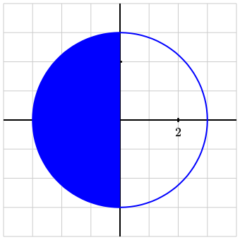
Let \(D\) be the region inside the unit circle centered at the origin, let \(R\) be the right half of \(D\text{,}\) and let \(B\) be the bottom half of \(D\text{.}\)

(a)

On three separate plots, graph and label the regions \(D\text{,}\) \(R\text{,}\) and \(B\text{.}\)

(b)

For each double integral below, decide without calculation whether the double integral is positive, negative, or zero. Write a sentence or two to explain your answer for each part.

\(\displaystyle \iint_D \; 1\; dA\)
\(\displaystyle \iint_D \; x \; dA\)
\(\displaystyle \iint_B \; x \; dA\)
\(\displaystyle \iint_R \; x \; dA\)
\(\displaystyle \iint_D \; x^2 \; dA\)
\(\displaystyle \iint_B \; 2-x^2 \; dA\)
\(\displaystyle \iint_R \; -e^x \; dA\)
\(\displaystyle \iint_B \; 1-e^y \; dA\)
\(\displaystyle \iint_D \; xy \; dA\)

Subsection 12.4.3 Horizontally and Vertically Simple Regions

The key idea to calculating double integrals using iterated integrals as shown in Section 12.3 and Preview Activity 12.4.1 is to slice the region of integration along a trace where one of the coordinates is held constant. We then express the range of the other coordinate in terms of an inequality. In this subsection, we will step away from double integrals for a short while to practice slicing two dimensional regions and stating corresponding inequalities in terms of each coordinate.

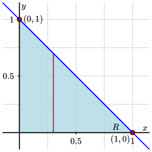
In Preview Activity 12.4.1, we considered a tetrahedron, which had as its base a triangular region \(R\) in the \(xy\)-plane. This region is shown in Figure 12.4.4.

described in detail following the image — Figure 12.4.4. The projection of \(T\) onto the \(xy\)-plane

Notice how different values of \(a\) provide different ranges of \(y\)-values for the portion of the \(x=a\) line segment that lies inside \(R\text{.}\) This is intrinsically linked with the fact that \(R\) is not a rectangular region, in contrast to the regions of integration from Section 12.3 which were all of the form \(a \leq x \leq b\) and \(c \leq y \leq d\) (with \(a,b,c,d\) constants).

These forms for the inequalities lead to a nice way to write the corresponding double integral as an iterated integral by considering the inner integral to evaluate the cross section area and the outer integral to sum the corresponding cross section volumes as the thickness of the slabs goes to zero.

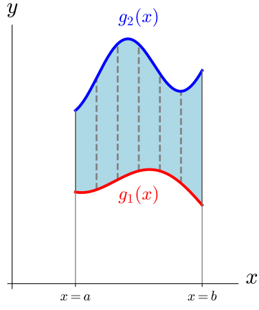
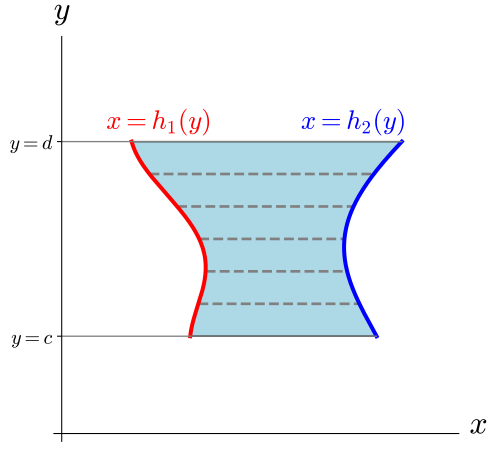
Not all two-dimensional regions can be immediately expressed using this idea of converting geometric slices to inequalities. The key characteristic that allows us to do this is a region must have the same upper and lower bound expressions for each slice.

Key Idea 12.4.5.

A region is called vertically simple if it can be described by a set of inequalities of the form

\begin{gather*} a \leq x \leq b\\ g_1(x) \leq y \leq g_2(x)\text{.} \end{gather*}

These inequalities correspond geometrically to the region in Figure 12.4.6.

A region is called horizontally simple if it can be described by a set of inequalities of the form

\begin{gather*} c \leq y \leq d\\ h_1(y) \leq x \leq h_2(y) \end{gather*}

which corresponds geometrically to the region in Figure 12.4.7.

A vertically simple region is one that can be split into vertical slices of the form \(x=\text{constant}\) for \(x\) in the interval \([a,b]\) where every vertical slice has the same upper and lower bound function: \(g_1(x) \leq y \leq g_2(x)\text{.}\) A horizontally simple region is one that can be split into horizontal slices of the form \(y=\text{constant}\) for \(y\) in the interval \([c,d]\) where every horizontal slice has the same upper (right) and lower (left) bound functions: \(h_1(x) \leq y \leq h_2(x)\text{.}\)

Example 12.4.8.

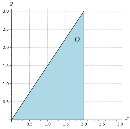
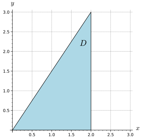
Let \(D\) be the triangular region in the \(xy\)-plane with vertices \((0,0)\text{,}\) \((2,0)\text{,}\) and \((2,3)\text{,}\) shown in Figure 12.4.9. We will determine if \(D\) is horizontally simple, vertically simple, or both. For simplicity, we refer to the three sides as follows:

the horizontal side from \((0,0)\) to \((2,0)\text{,}\)
the vertical side from \((2,0)\) to \((2,3)\text{,}\) and
the diagonal side from \((0,0)\) to \((2,3)\text{.}\)

(a)

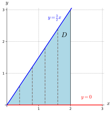
A vertical line has equation \(x=\text{constant}\text{.}\) We must determine if every vertical slice in the region \(D\) has the same upper and lower bounds, which may depend on the value of \(x\text{.}\) Geometrically, we are asking if the region \(D\) has the same functions as the top and bottom of the region for each value of \(x\text{.}\)

Several vertical slices in the region \(D\) are shown in Figure 12.4.10 where you can see that the lower bound of the \(y\)-value for every vertical slice is given by \(y=0\text{.}\) The upper bound of the \(y\)-value for every vertical slice is given by \(y=\frac{3}{2} x\text{.}\) Algebraically, for any constant value \(k\) in the interval \([0,2]\text{,}\) the following statement describes the vertical slices of the region \(D\text{:}\)

\begin{equation*} \text{Along }x=k\text{ the }y\text{-coordinates go from }0\text{ to }\frac{3}{2}k \end{equation*}

which corresponds to the inequalities

\begin{equation*} 0\leq x \leq 2 \quad \quad 0 \leq y \leq \frac{3}{2} x \end{equation*}

as a description for \(D\text{.}\) Thus, the region \(D\) is vertically simple.

(b)

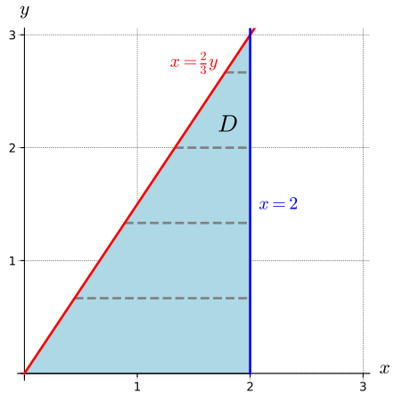
A horizontal line has equation \(y=k\) where \(k\) is a constant. We must determine if every horizontal slice in the region \(D\) has the same upper and lower bounds, which may depend on the value of \(y\text{.}\) Geometrically, this corresponds to having the same functions of \(y\) as the right and left boundaries of the region.

Several horizontal slices in the region \(D\) are shown in Figure 12.4.11 where you can see that the lower bound of the \(x\)-value for every horizontal slice is given by \(x=\frac{2}{3} y\text{.}\) The upper bound of the \(x\)-value for every horizontal slice is given by \(x=2\text{.}\) Algebraically, for any constant value \(k\) in the interval \([0,3]\text{,}\) the following statement describes the horizontal slices of the region \(D\text{:}\)

\begin{equation*} \text{Along }y=k\text{ the }x\text{-coordinates go from }\frac{2}{3} k\text{ to }2 \end{equation*}

which corresponds to the inequalities

\begin{equation*} 0\leq y \leq 3 \quad \quad \frac{2}{3} \leq y \leq 2 x \end{equation*}

as a description for \(D\text{.}\) Thus, the region \(D\) is horizontally simple.

This example shows that just because a region is vertically simple does not mean that it is not horizontally simple as well. In general, a two-dimensional region can be any of the following

horizontally simple (but not vertically simple),
vertically simple (but not horizontally simple),
both horizontally simple and vertically simple, or
neither horizontally simple or vertically simple.

As we will see later, switching the description of a region that is both horizontally simple and vertically simple can make the algebra of evaluating an iterated integral easier.

Example 12.4.12.

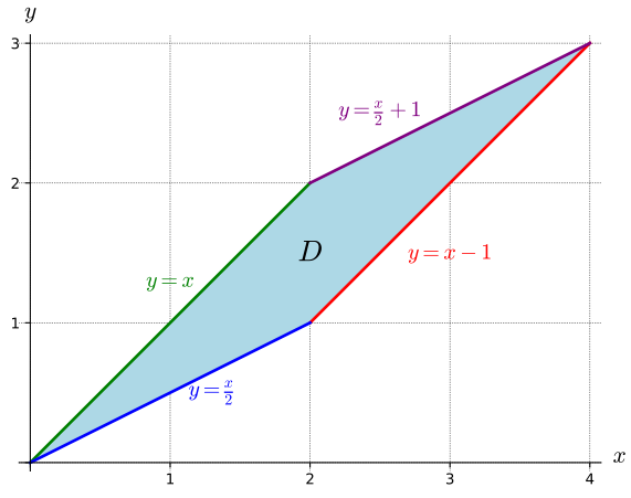
In this example, we will look at region that is neither horizontally or vertically simple. Let \(D\) be the parallelogram with vertices \((0,0)\text{,}\) \((2,1)\text{,}\) \((4,3)\text{,}\) and \((2,2)\) as shown in Figure 12.4.13. You should take a moment to verify each of the equations for the lines that bound \(D\text{.}\)

(a)

If we try to look at \(D\) along vertical slices of the form \(x=k\text{,}\) different values of \(k\) will have different upper and lower bounds. For instance, the default \(k\) value of 0.5 shown in Figure 12.4.14 is a vertical segment with lower bound at the point \(\left(k,\frac{k}{2}\right)\) and upper bound at the point \(\left(k,k\right)\text{.}\) Use the slider at the top of Figure 12.4.14 to change the value of \(k\) to a number greater than 2. For such values, the vertical slice of \(D\) along \(x=k\) will have lower bound \(\left(k,k-1\right)\) and upper bound \(\left(k,\frac{k}{2}+1\right)\text{.}\) Because the upper or lower bound functions depend on the location of a vertical slice, \(D\) is not vertically simple.

The region \(D\) shown in Figure 12.4.13 along with a vertical slice. The position of the vertical slice can be adjusted with a slider labeled \(k\text{.}\) The coordinates of the points at the bottom and top of the vertical slice are shown (in terms of \(k\)) and change as the slider is moved.

Figure 12.4.14. The region \(D\) with vertical slices that change upper and lower bounds depending on the value of \(x=k\)

(b)

If we try to look at \(D\) along horizontal slices of the form \(y=k\text{,}\) different values of \(k\) will have different upper and lower bounds. For instance, the default \(k\) value of 0.5 shown in Figure 12.4.15 is a vertical segment with lower bound at the point \(\left(k,k\right)\) and upper bound at the point \(\left(2k,k\right)\text{.}\) Use the slider at the top of Figure 12.4.15 to change the value of \(k\) to a number greater than 1. You can see that for \(k\) values between 1 and 2, the upper bound on the horizontal segment becomes \(\left(k-1,k\right)\) and for \(k\) values above 2, the lower bound also changes to \(\left(\frac{k}{2}+1,k\right)\text{.}\) Because the upper or lower bound functions depend on the location of the horizontal slice, \(D\) is not horizontally simple.

The region \(D\) shown in Figure 12.4.13 along with a horizontal slice. The position of the horizontal slice can be adjusted with a slider labeled \(k\text{.}\) The coordinates of the points at the left and right of the horizontal slice are shown (in terms of \(k\)) and change as the slider is moved.

Figure 12.4.15. The region \(D\) with horizontal slices that change upper and lower bounds depending on the value of \(y=k\)

Activity 12.4.3.

In this activity, we will break the region \(D\) from Example 12.4.12 into smaller regions which are horizontally or vertically simple.

(a)

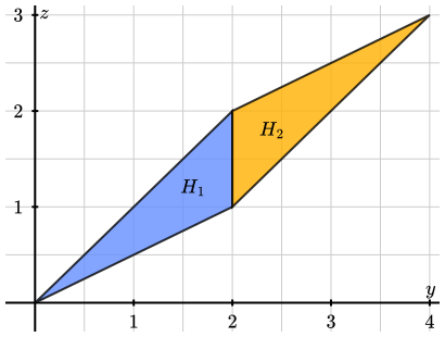
In Figure 12.4.16, the region \(D\) is broken into two regions, \(V_1\) and \(V_2\text{.}\) Give inequalities for each of \(V_1\) and \(V_2\) that shows each region is vertically simple.

(b)

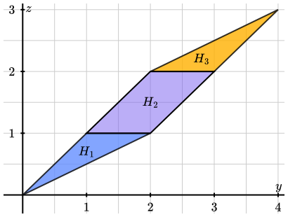
In Figure 12.4.17, the region \(D\) is broken into three regions \(H_1\text{,}\) \(H_2\text{,}\) and \(H_3\text{.}\) Give inequalities for each of \(H_1\text{,}\) \(H_2\text{,}\) and \(H_3\) that shows that each region is horizontally simple.

In single variable calculus, we were able to split integrals into multiple parts. The integral of \(f(x)\) over \([a,b]\) could be split to subintervals separately:

\begin{equation*} \int^b_a f(x) \, dx = \int_a^c f(x) \, dx + \int_c^b f(x) \, dx\text{.} \end{equation*}

Similarly, we can split a region of integration for a double integral into subregions. If a region \(R\) can be split into two nonoverlapping regions \(R_1\) and \(R_2\text{,}\) then

\begin{equation*} \iint_R f(x,y) \, dA = \iint_{R_1} f(x,y) \, dA+\iint_{R_2} f(x,y) \, dA\text{.} \end{equation*}

This property is useful for a region similar to Figure 12.4.17 where \(D\) is split into parts \(H_1\text{,}\) \(H_2\text{,}\) and \(H_3\) because

\begin{equation*} \iint_D f(x,y) \, dA = \iint_{H_1} f(x,y) \, dA+\iint_{H_2} f(x,y) \, dA+\iint_{H_3} f(x,y) \, dA\text{,} \end{equation*}

where each of the double integrals on the right can be written as an iterated integral using a horizontally simple description.

The process for describing a two-dimensional region as horizontally or vertically simple is exactly the procedure needed to set up an iterated integral to evaluate a double integral.

Key Idea 12.4.18.

If a vertically simple region \(D\) can be described by the inequalities \(a \leq x \leq b\) and \(g_1(x) \leq y \leq g_2(x)\text{,}\) where \(g_1(x)\) and \(g_2(x)\) are functions of only \(x\text{,}\) then the double integral can be written as an iterated integral in the following way

\begin{equation*} \iint_D f(x,y) \, dA = \int_{x=a}^{x=b} \int_{y=g_1(x)}^{y=g_2(x)} f(x,y) \, dy \, dx\text{.} \end{equation*}

Alternatively, if a horizontally simple region \(D\) is described by the inequalities \(c \leq y \leq d\) and \(h_1(y) \leq x \leq h_2(y)\text{,}\) where \(h_1(y)\) and \(h_2(y)\) are functions of only \(y\text{,}\) then the double integral can be written as an iterated integral in the following way

\begin{equation*} \iint_D f(x,y) \, dA = \int_{y=c}^{y=d} \int_{x=h_1(y)}^{x=h_2(y)} f(x,y) \, dx \, dy\text{.} \end{equation*}

Proof.

We will make a brief argument using the Classic Calculus Approach to give an outline for a proof of this result. We will visualize the double integral with a region similar to the one used in the Preview Activity, as shown in Figure 12.4.19. Remember that we will have a region of integration given by the inequalities \(a \leq x \leq b\) and \(g_1(x) \leq y \leq g_2(x)\text{,}\) where \(g_1(x)\) and \(g_2(x)\) are functions of only \(x\)

Coordinate axes for \(xyz\)-space showing a solid region over the triangle with vertices \((0,0,0)\text{,}\) \((1,0,0)\text{,}\) and \((0,1,0)\text{.}\)

Figure 12.4.19. The double integral \(\iint_R f(x,y) dA\) visualized as the volume between the \(xy\)-plane and the surface given by \(z=f(x,y)\text{,}\) shown in pink, over the region \(R\text{,}\) shown in blue

For Step 1 of the Classic Calculus Approach, we approximate this double integral with \(n\) prisms of equal width along constant values of \(x\) as shown in Figure 12.4.20. The width of these \(n\) equal width prisms will be \(\Delta x=\frac{b-a}{n}\text{.}\) These prisms will involve the cross sectional area of our volume at the following values of \(x\text{:}\) \(x_0=a,x_1=a+\Delta x, \ldots , x_i = a+i \Delta x, \ldots, x_{n-1}=a+(i-1)\Delta x\text{.}\)

Coordinate axes for \(xyz\)-space showing a solid region over the triangle with vertices \((0,0,0)\text{,}\) \((1,0,0)\text{,}\) and \((0,1,0)\text{.}\)

Figure 12.4.20. The double integral \(\iint_R f(x,y) dA\) approximated by prisms along constant values of \(x\)

The cross sectional area of the volume at \(x=a\) is given by

\begin{equation*} CSA(a)=\int_{y=g_1(a)}^{y=g_2(a)} f(a,y) dy\text{.} \end{equation*}

Note that this takes the height of the surface on this slice and integrates over only the relevant range of \(y\)-values. Our approximation for Step 1 of the Classic Calculus Approach is given by

\begin{equation*} \iint_R f(x,y) dA \approx \sum_{n=0}^{n-1} \text{CSA}(a) \Delta x \end{equation*}

Note that this approximation already accomplishes Step 2 of the Classic Calculus Approach since a smaller scale means that we have an increase in \(n\text{,}\) the number of cross section prisms, which decreases \(\Delta x\text{,}\) the width of the prisms.

Applying a limit in Step 3 of our approximation yields

\begin{equation*} \iint_R f(x,y) dA =\lim_{n\to \infty} \sum_{n=0}^{n-1} \text{CSA}(x_i) \Delta x\text{,} \end{equation*}

which you may recognize as a definite integral. In particular,

\begin{equation*} \iint_R f(x,y) dA =\int_{x=a}^{x=b} \text{CSA}(x) dx\text{.} \end{equation*}

We can substitute this in our expression for \(\text{CSA}(x)\) to get

\begin{equation*} \iint_R f(x,y) dA =\int_{x=a}^{x=b} \left[ \int_{y=g_1(x)}^{y=g_2(x)} f(x,y) dy \right] dx\text{.} \end{equation*}

Note that when we substituted in our expression for the cross sectional area integral, we used the variable \(x\) since that corresponds to the value/variable used in the larger expression. The other result with prisms along constant values of \(y\) has a very analogous argument but does not offer any additional illumination, so we omit this discussion.

The structure of an iterated integral that will be used to evaluate a double integral must satisfy the following:

The limits on the inner integral must be constants or expressed only in terms of the outer variable—that is, if the inner integral is with respect to \(y\text{,}\) then its limits may only involve \(x\) and constants.
The limits on the outer integral must be constants.

The next activity gives you the opportunity to practice describing regions as horizontally simple, vertically simple, both, or neither. It then presents some iterated integrals and asks you to determine if they meet the requirements above to correspond to a double integral.

Activity 12.4.4.

(a)

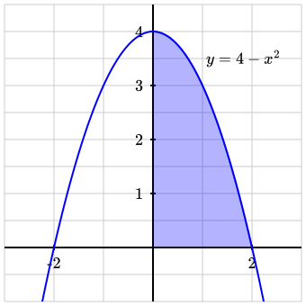
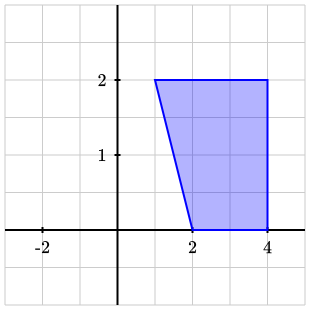
For each region shown below, state whether the region is vertically simple, horizontally simple, both, or neither. State the appropriate inequalities to justify when a region is vertically simple or horizontally simple.

(b)

For each of the interated integrals below, write out the bounds of the integral as a set of inequalities. Use these inequalities to decide if the bounds of the iterated integrals make sense to compute a double integral. For any iterated integral with bounds that do not make sense as a double integral, explain your reasoning in a couple of sentences. For any bounds of an iterated integral that does make sense as a double integral, sketch a plot of the associated region of integration.

(i)

\(\displaystyle \int_0^1 \int_1^x f(x,y) \; dy \; dx \)

(ii)

\(\displaystyle \int_0^1 \int_1^y f(x,y) \; dy \; dx\)

(iii)

\(\displaystyle \int_0^1 \int_x^y f(x,y) \; dy \; dx\)

(iv)

\(\displaystyle \int_0^1 \int_x^1 f(x,y) \; dy \; dx\)

Subsection 12.4.4 Double Integrals Evaluated as Iterated Integrals

We now turn our attention to using iterated integrals to evaluate double integrals. This is a powerful algebraic tool that we will use throughout the remainder of this chapter, but as the second part of Activity 12.4.4 showed, not every iterated integral that can be written down is meaningful in the sense of evaluating double integrals. As you read the rest of this section, pay careful attention to understanding the meaning behind the computations.

Example 12.4.22.

Let \(f(x,y) = x^2y\) be defined on the triangle \(D\) with vertices \((0,0)\text{,}\) \((2,0)\text{,}\) and \((2,3)\) as shown in Figure 12.4.23. This is the same region we described in Example 12.4.8. In this example, we will use the inequalities from that example that described the region as vertically simple to set up and evaluate an iterated integral that gives the value of the double integral.

(a)

We use the inequalities from Example 12.4.8 that correspond to our vertically simple description:

\begin{equation*} \text{Along }x=k\text{, the }y\text{-coordinates go from }0\text{ to }\frac{3}{2}k\text{,} \end{equation*}

which corresponds to the inequalities

\begin{equation*} 0\leq x \leq 2 \quad \quad 0 \leq y \leq \frac{3}{2} x\text{.} \end{equation*}

Using these inequalities corresponds to integrating with respect to \(y\) first. That is, the variable in the inner integral is \(y\text{.}\)

Therefore,

\begin{equation*} \iint_D x^2y \, dA = \int_{x=0}^{x=2} \int_{y=0}^{y = \frac32 x} x^2y \, dy \, dx\text{.} \end{equation*}

We evaluate the iterated integral by applying the Fundamental Theorem of Calculus first to the inner integral followed by the outer one. To do this, let’s go carefully step-by-step and first evaluate the inner integral on its own. To do this, remember that, much like with computing partial derivatives, we treat \(x\) as a constant since we are integrating with respect to \(y\text{.}\) Therefore, we find an antiderivative with respect to \(y\) for the integrand proceed using the Fundamental Theorem of Calculus as follows:

\begin{equation} \int_{y=0}^{y=\frac32 x} x^2y \, dy = \left[x^2 \cdot \frac{y^2}{2}\right]\restrict{y=0}{y=\frac32 x} = \frac{9}{8}x^4\tag{12.4.2} \end{equation}

Using this to complete the evaluation of the interated integral, we now have

\begin{align*} \int_{x=0}^{x=2} \int_{y=0}^{y=\frac32 x} x^2y \, dy \, dx \amp = \int_{x=0}^{x=2} \frac{9}{8}x^4\, dx\\ \amp = \frac{9}{8}\frac{x^5}{5}\restrict{x=0}{x=2}\\ \amp = \left(\frac{9}{8}\right) \left(\frac{32}{5}\right)\\ \amp = \frac{36}{5}\text{.} \end{align*}

Figure 12.4.24 provides an opportunity to visualize both the double integral and the iterated integral.

The double integral of \(f(x,y)=x^2y\) over the region \(D\) can be seen as the volume of the solid below the surface \(z=f(x,y)\) and above the \(xy\)-plane on the region \(D\text{.}\) This is shown as the pink volume in Figure 12.4.24. We can also use each of the iterated integrals to visualize the result.
The inner integral, which we evaluated in (12.4.2) to have value \(\frac{9}{8}x^4\text{,}\) corresponds to the area of a cross section along a slice with a fixed \(x\)-value, as shown by the blue cross section in Figure 12.4.24. The result of the inner integral changes depending on which \(x\)-value is used. Move the slider at the top of Figure 12.4.24 to change the \(x\)-value at which the slice of the solid is taken and observe that the area of the cross section increases as \(x\) increases.

A three-dimensional plot of a solid in \(xyz\)-space. The solid is bounded below by the \(xy\)-plane, and its base is the triangular region \(D\) with vertices \((0,0)\text{,}\) \((2,0)\text{,}\) and \((2,3)\text{.}\) The upper surface of the solid rises from the origin in a curved manner and is determined by the graph of the function \(f(x,y)=x^2y\text{.}\) A cross section of the solid parallel to the \(yz\)-plane is highlighted with a slider that can adjust the \(x\)-value at which the cross section is located.

Figure 12.4.24. A plot of the volume below \(f(x,y)\) over the region \(D\) with a highlighted cross section for \(x=k\)

(b)

We conclude this example by discussing what the function obtained by evaluating the inner integral in the iterated integrals tells us geometrically. Evaluating the inner integral gave us the function \(\frac{9}{8}x^4\text{.}\) Figure 12.4.25 shows a plot of this function on the interval \([0,2]\text{.}\) The value of this function for a specific value of \(x\) gives the area of the cross section of the original solid at that location. Move the slider in the figure to see the value of this area function at different values of \(x\text{.}\) As you noticed when examining Figure 12.4.24, the cross sections with \(x\) close to zero are very small, and the areas of the cross sections increase as \(x\) increases.

A two-dimensional plot of a shaded region. The region is bounded below by the horizontal axis, which is labeled \(x\text{.}\) The vertical axis is labeled Area. The upper boundary of the region is a curve that contains the points \((0,0)\) and \((2,18)\text{.}\) Between these points, the curve is concave up. There is a slider that allows adjustment of the position of a vertical line segment inside the region.

Figure 12.4.25. A plot of \(\frac{9}{8}x^4\) on the interval \([0,2]\)

We know from single-variable calculus that evaluating the outer integral in the iterated integral must give the area under the graph in Figure 12.4.25. One of the interpretations we have been considering of a double integral tells us that this ultimately yields the volume of the three-dimensional solid. This makes sense because the values of the function being integrated in the outer integral are areas of cross sections.

Activity 12.4.5.

Let \(D\) be the triangular region with vertices \((0,0)\text{,}\) \((4,0)\text{,}\) and \((0,2)\text{.}\) Consider the double integral \(\displaystyle{\iint_D (4-x-2y) \, dA}\text{.}\)

(a)

Draw and label a plot of \(D\) with relevant cross sections for a vertically simple description. Give the inequalities that show \(D\) is vertically simple.

(b)

Write the double integral as an iterated integral of the form \(\displaystyle \iint_D (4-x-2y) \, dy \, dx\text{,}\) including correct bounds on the integral.

(c)

Evaluate the iterated integrals from the previous part. Write a sentence describing at least one interpretation of the meaning of the value of the double integral.

The region we considered as vertically simple in Example 12.4.22 was shown in Example 12.4.8 to be both vertically simple and horizontally simple. We will now see that it is also possible to set up an iterated integral for the double integral using the horizontally simple description of the region.

Example 12.4.26.

Consider again the function \(f(x,y) = x^2y\) on the triangle \(D\) with vertices \((0,0)\text{,}\) \((2,0)\text{,}\) and \((2,3)\) as shown in Figure 12.4.23. This is the same region we described as both vertically simple and horizontally simple in Example 12.4.8. In Example 12.4.22, we set up an iterated integral for \(\iint_D f(x,y)\, dA\) using the vertically simple description of \(D\text{.}\) In this example, we will use the horizontally simple description of \(D\) to write another iterated integral that computes thd double integral.

(a)

We will use the inequalities from Example 12.4.8 that correspond to the horizontally simple description of \(D\text{:}\)

\begin{equation*} \text{Along }y=k\text{, the }x\text{-coordinates go from }\frac{2}{3}k\text{ to }2 \end{equation*}

This description corresponds to the inequalities

\begin{equation*} 0\leq y \leq 3 \quad \quad \frac{2}{3}y \leq x \leq 2\text{.} \end{equation*}

Using these inequalities corresponds to integrating with respect to \(x\) in the inner integral of the iterated integral. That is, the variable in the inner integral is \(x\) and we treat \(y\) as a constant when antidifferentiating.

Therefore we can write the double integral as a \(dx\, dy\) iterated integral in the form

\begin{equation*} \iint_D x^2y \, dA = \int_{y=0}^{y=3} \int_{x=\frac{2}{3} y}^{x=2} x^2y \, dx \, dy\text{.} \end{equation*}

We can now evaluate the resulting iterated integral as before by twice applying the Fundamental Theorem of Calculus. In the inner integral, we treat \(y\) as a constant and integrate with respect to \(x\text{.}\) When we do so, we find that

\begin{align*} \int_{y=0}^{y=3} \int_{x=\frac{2}{3}y}^{2} x^2y \, dx \, dy \amp = \int_{y=0}^{y=3} \left[ \frac{x^3}{3}\cdot y \right]\restrict{x=\frac{2}{3}y}{x=2} \, dx\\ \amp = \int_{y=0}^{y=3} \left[ \frac{8}{3}y - \frac{8}{81}y^4 \right] \, dy\\ \amp = \left[ \frac{8}{3}\frac{y^2}{2} - \frac{8}{81}\frac{y^5}{5}\right] \restrict{y=0}{y=3}\\ \amp = \left(\frac{8}{3}\right) \left(\frac{9}{2}\right) - \left(\frac{8}{81}\right) \left(\frac{243}{5}\right)\\ \amp = 12 - \frac{24}{5}\\ \amp = \frac{36}{5}\text{.} \end{align*}

In Figure 12.4.27, you can see the same solid as before in pink. The volume of this solid is the value of the double integral. In this example, we used a horizontally simple description which means the slices correspond to constant values of \(y\text{.}\) A cross section along a constant \(y\)-value is shown in blue in the figure. Use the slider at the top of Figure 12.4.27 to see how the size of cross section changes with respect to \(y\text{.}\) Notice how as \(y\) increases, the area of the cross section first increases and then decreases.

A three-dimensional plot of a solid in \(xyz\)-space. The solid is bounded below by the \(xy\)-plane, and its base is the triangular region \(D\) with vertices \((0,0)\text{,}\) \((2,0)\text{,}\) and \((2,3)\text{.}\) The upper surface of the solid rises from the origin in a curved manner and is determined by the graph of the function \(f(x,y)=x^2y\text{.}\) A slice of the solid parallel to the \(xz\)-plane is shown with a slider that can adjust the \(y\)-value at which the slice is located.

Figure 12.4.27. A plot of the solid below \(f(x,y)\) over the region \(D\)

(b)

As with our previous consideration of this double integral, we conclude this example by examining what the function obtained by evaluating the inner integral in the iterated integrals tells us geometrically. In part a, the inner integral evaluated to \(\frac{8}{3}y-\frac{8}{81}y^4\text{.}\) The relevant \(y\)-values satisfy \(0\leq y\leq 3\text{.}\) In Figure 12.4.28, we show a plot of this function on the interval \([0,3]\) along with a slider. Moving the slider corresponds to changing the location of the cross section in Figure 12.4.27. In Figure 12.4.28, it helps illustrate the value of the inner integral at that value of \(y\text{.}\) The value of this function for a particular value of \(y\) is the area of the cross section of the solid at that \(y\)-position. Therefore, just as you visually observed by moving the slider in Figure 12.4.27, the cross section is small for \(y\) values near \(0\) or \(3\text{.}\) The area of the cross section is largest when the \(y\)-value is slightly larger than \(2\text{.}\) This figure demonstrates how the function obtained by evaluating the inner integral is the function giving the area of a cross section for a constant value of \(y\text{.}\)

A two-dimensional plot of a shaded region. The region is bounded below by the horizontal axis, which is labeled \(y\text{.}\) The vertical axis is labeled Area. The upper boundary of the region is a curve that contains the points \((0,0)\) and \((3,0)\text{.}\) Between these points, the curve is concave up until approximately \(y=1.5\) and then concave down. There is a slider that allows adjustment of the position of a vertical line segment inside the region.

Figure 12.4.28. A plot of \(\frac{8}{3}y-\frac{8}{81}y^4\) on the interval \([0,3]\)

Recall that evaluating the outer integral in part a finds the area of the shaded region in Figure 12.4.28. Remembering that the height of the function’s graph in that plot is the area of a cross section tells us that the outer integral corresponds to accumulating area. This leads to the value of the double integral measuring the volume of the solid.

We have now seen that in a situation where \(D\) can be described as both horizontally simple and vertically simple, we can set up an iterated integral in either order. If we can reasonably evaluate the iterated integral in either order, then the iterated integrals yield the same value in each case. However, there are times where finding an antiderivative to evaluate the inner integral may be easier in one order than the other.

The process of switching between a vertically simple description and a horizontally simple description for the region of integration is often called switching the order of integation because the corresponding iterated integrals used to calculate a double integral will have the order in which you integrate these variables switched.

The possible meanings of a double integral \(\iint_D f(x,y)\, dA\) over a non-rectangular region \(D\) are the same as those we stated for a double integral over a rectangular region:

The volume of the solids the graph of \(f\) bounds above the \(xy\)-plane over the region \(D\) minus the volume of the solids the graph of \(f\) bounds below the \(xy\)-plane under the region \(D\text{.}\)
If \(f(x,y)\) is the density of a substance over a region \(D\text{,}\) then the double integral of \(f\) over \(D\) will measure the total amount of the substance in \(D\text{.}\)
Dividing the double integral by the area of \(D\) gives the average value of \(f\) over the region \(D\text{.}\)

The next activity asks you to return to the function and triangular region considered in Activity 12.4.5 but to set up an iterated integral from the perspective of the region being horizontally simple.

Activity 12.4.6.

Let \(D\) be the triangular region with vertices \((0,0)\text{,}\) \((4,0)\text{,}\) and \((0,2)\text{.}\) Consider the double integral \(\displaystyle{\iint_D (4-x-2y) \, dA}\text{.}\)

(a)

Draw and label a plot of \(D\) with relevant cross sections for a horizontally simple description. Give the inequalities that show \(D\) is horizontally simple.

(b)

Write the double integral as an iterated integral of the form \(\iint_D (4-x-2y) \, dx \, dy\text{,}\) include correct bounds on the integral.

(c)

Evaluate the iterated integral above, and verify that you get the same value as in Activity 12.4.5.

The next activity explores a region of integration with non-linear sides, given as bounds in an iterated integral. You will also switch the order of integration, evaluate whichever order is most convinient, and finally interpret the result as the average value.

Activity 12.4.7.

Consider the iterated integral \(\displaystyle\int_{x=0}^{x=1} \int_{y=x}^{y=\sqrt{x}} (4x+10y) \, dy \, dx\text{.}\) Remember that not every iterated integral makes sense as a double integral, so as you proceed through this activity, pause to think about why this iterated integral does correspond to a double integral.

(a)

Sketch the region of integration \(D\) for which

\begin{equation*} \iint_D (4x + 10y) \, dA = \int_{x=0}^{x=1} \int_{y=x}^{y=\sqrt{x}} (4x+10y) \, dy \, dx\text{.} \end{equation*}

(b)

Determine the equivalent iterated integral that results from integrating in the opposite order (\(dx \, dy\text{,}\) instead of \(dy \, dx\)). That is, determine limits of integration for which

\begin{equation*} \iint_D (4x + 10y) \, dA = \int_{y=?}^{y=?} \int_{x=?}^{x=?} (4x+10y) \, dx \, dy\text{.} \end{equation*}

(c)

Evaluate whichever one of the two iterated integrals above you find easier to compute. Explain what the value means in at least one of the interpretations of Key Idea 12.2.8.

(d)

Set up and evaluate a single definite integral to determine the exact area \(A(D)\) of \(D\text{.}\)

(e)

Determine the exact average value of \(f(x,y) = 4x + 10y\) over \(D\text{.}\)

We mentioned earlier that sometimes antidifferentiating in an iterated integral is difficult. To illustrate this, Exercise 12.4.5.23 asks you to consider

\begin{equation*} \displaystyle\int_{x=0}^{x=4} \int_{y=x/2}^{y=2} e^{y^2} \, dy \, dx \end{equation*}

and explores how how switching the order of integration can sometimes yield a significantly easier iterated integral to evaluate algebraically.

Summary

For a double integral \(\displaystyle{\iint_D f(x,y) \, dA}\text{,}\) we can write appropriate iterated integrals if the region \(D\) is either horizontally or vertically simple.
- A horizontally simple region is described by the inequalities \(c \leq y \leq d\) and \(h_1(y) \leq x \leq h_2(y)\text{.}\)
- A vertically simple region is described by \(a \leq x \leq b\) and \(g_1(x) \leq y \leq g_2(x)\text{.}\)
🔗
🔗
In an iterated double integral, the limits on the outer integral must be constants while the limits on the inner integral must be constants or in terms of only the remaining variable. In other words, an iterated integral corresponding to a double integral has one of the following forms (which result in the same value):

\begin{equation*} \int_{x=a}^{x=b} \int_{y=g_1(x)}^{y=g_2(x)} f(x,y) \, dy \, dx, \end{equation*}

where \(g_1=g_1(x)\) and \(g_2=g_2(x)\) are functions of \(x\) only and the region \(D\) is described by the inequalities \(a \leq x \leq b\) and \(g_1(x) \leq y \leq g_2(x)\) or

\begin{equation*} \int_{y=c}^{y=d} \int_{x=h_1(y)}^{x=h_2(y)} f(x,y) \, dx \, dy, \end{equation*}

where \(h_1=h_1(y)\) and \(h_2=h_2(y)\) are functions of \(y\) only and the region \(D\) is described by the inequalities \(c \leq y \leq d\) and \(h_1(y) \leq x \leq h_2(y)\text{.}\)

Exercises 12.4.5 Exercises

1.

Decide, without calculation, if each of the integrals below are positive, negative, or zero. Let D be the region inside the unit circle centered at the origin. Let T, B, R, and L denote the regions enclosed by the top half, the bottom half, the right half, and the left half of unit circle, respectively.

\(\displaystyle \displaystyle \iint\limits_B (y^3 + y^5) \, dA\)
\(\displaystyle \displaystyle \iint\limits_T (y^3 + y^5) \, dA\)
\(\displaystyle \displaystyle \iint\limits_D (y^3 + y^5) \, dA\)
\(\displaystyle \displaystyle \iint\limits_L (y^3 + y^5) \, dA\)
\(\displaystyle \displaystyle \iint\limits_R (y^3 + y^5) \, dA\)

2.

Match the following integrals with the verbal descriptions of the solids whose volumes they give. Put the letter of the verbal description to the left of the corresponding integral.

\(\displaystyle \displaystyle \int_{-1}^{1}\!\!\int_{-\sqrt{1-x^{2}}}^{\sqrt{1-x^{2}}} 1 - x^{2} - y^{2}\: dy dx\)
\(\displaystyle \displaystyle \int_{-2}^{2}\!\!\int_{4}^{4 + \sqrt{4-x^{2}}} 4x + 3y \: dy dx\)
\(\displaystyle \displaystyle \int_{0}^{\frac{1}{\sqrt{3}}}\!\!\int_{0}^{\frac{1}{2}\sqrt{1-3y^{2}}} \sqrt{1 -4x^{2} - 3y^{2}} \: dx dy\)
\(\displaystyle \displaystyle \int_{0}^{1}\!\!\int_{y^{2}}^{\sqrt{y}} 4x^{2} + 3y^{2} \: dx dy\)
\(\displaystyle \displaystyle \int_{0}^{2}\!\!\int_{-2}^{2} \sqrt{4 - y^{2}} \: dy dx\)

One eighth of an ellipsoid.
Solid under an elliptic paraboloid and over a planar region bounded by two parabolas.
Solid under a plane and over one half of a circular disk.
One half of a cylindrical rod.
Solid bounded by a circular paraboloid and a plane.

3.

In evaluating a double integral over a region \(D\text{,}\) a sum of iterated integrals was obtained as follows:

\begin{equation*} \iint_D f(x,y)\, dA = \int_0^{2} \int_0^{(5/2)y} f(x,y)\, dx dy + \int_{2}^{7} \int_0^{7-y} f(x,y)\, dx dy \, . \end{equation*}

Sketch the region \(D\) and express the double integral as an iterated integral with reversed order of integration.

\(\displaystyle \int_a^b \int_{g_1(x)}^{g_2(x)} f(x,y)\, dy dx\)

\(a =\) \(b =\)

\(g_1(x) =\) \(g_2(x) =\)

4.

Evaluate the integral

\begin{equation*} \int_0^{1}\int_y^{1} \sin(x^2)\ dx\,dy \end{equation*}

by reversing the order of integration.

With order reversed,

\begin{equation*} \int_a^b\int_c^d \sin(x^2)\ dy\,dx, \end{equation*}

where \(a =\) , \(b =\) , \(c =\) , and \(d =\) .

Evaluating the integral, \(\int_0^{1}\int_y^{1} \sin(x^2)\ dx\,dy =\)

5.

Evaluate the iterated integral \(\displaystyle \int_0^{3} \int_0^{e^v} \!\! \sqrt{1+e^v} \,dw\, dv.\)

Answer:

6.

Evaluate the double integral \(\displaystyle I = \int\!\!\int_{\mathbf{D}} xy \: d\!A\) where \(\mathbf{D}\) is the triangular region with vertices \((0, 0), (3, 0), (0, 3)\text{.}\)

7.

Evaluate the double integral \(\displaystyle I = \int\!\!\int_{\mathbf{D}} xy \: d\!A\) where \(\mathbf{D}\) is the triangular region with vertices \((0, 0), (4, 0), (0, 1)\text{.}\)

8.

Evaluate the integral by reversing the order of integration.

\(\int_{0}^{1}\!\!\int_{7y}^{7} e^{x^{2}} \, dx dy =\)

9.

Consider the integral \(\displaystyle \int_0^7 \int_0^{\sqrt{49-y}} f(x,y) dx dy\text{.}\) If we change the order of integration we obtain the sum of two integrals:

\(\displaystyle \int_a^b \int_{g_1(x)}^{g_2(x)} f(x,y) dy dx + \displaystyle \int_c^d \int_{g_3(x)}^{g_4(x)} f(x,y) dy dx\)

\(a =\) \(b =\)

\(g_1(x) =\) \(g_2(x) =\)

\(c =\) \(d =\)

\(g_3(x) =\) \(g_4(x) =\)

10.

The region \(W\) lies below the surface \(f(x,y) = 4 e^{-(x-1)^2-y^2}\) and above the disk \(x^2+y^2\le 4\) in the \(xy\)-plane.

(a) Think about what the contours of \(f\) look like. You may want to using \(f(x,y)=1\) as an example. Sketch a rough contour diagram on a separate sheet of paper.

(b) Write an integral giving the area of the cross-section of \(W\) in the plane \(x=1\text{.}\)

Area = \(\int_a^b\) \(d\),

where \(a =\) and \(b =\)

(c) Use your work from (b) to write an iterated double integral giving the volume of \(W\text{,}\) using the work from (b) to inform the construction of the inside integral.

Volume = \(\int_a^b\int_c^d\) \(d\) \(d\),

where \(a =\) , \(b =\) \(c =\) and \(d =\)

11.

Set up a double integral in rectangular coordinates for calculating the volume of the solid under the graph of the function \(f(x,y) = 16-x^{2}-y^{2}\) and above the plane \(z = 7\text{.}\)

Instructions: Please enter the integrand in the first answer box. Depending on the order of integration you choose, enter dx and dy in either order into the second and third answer boxes with only one dx or dy in each box. Then, enter the limits of integration.

\(\displaystyle \int_A^B \int_C^D\)

A =

B =

C =

D =

12.

Find the volume of the solid bounded by the planes x = 0, y = 0, z = 0, and x + y + z = 2.

13.

A pile of earth standing on flat ground has height 9 meters. The ground is the xy-plane. The origin is directly below the top of the pile and the z-axis is upward. The cross-section at height z is given by \(x^2 + y^2 = 9 - z\) for \(0 \leq z \leq 9\text{,}\) with \(x, y,\) and \(z\) in meters.

(a) What equation gives the edge of the base of the pile?

\(\displaystyle x + y = 3\)
\(\displaystyle x + y = 9\)
\(\displaystyle x^2 + y^2 = 3\)
\(\displaystyle x^2 + y^2 = 9\)
None of the above

(b) What is the area of the base of the pile?

\(\displaystyle x^2 + y^2 = 8\)
\(\displaystyle x^2 + y^2 = \sqrt{1}\)
\(\displaystyle x^2 + y^2 = 64\)
\(\displaystyle x^2 + y^2 = 1\)
None of the above

(d) What is the area of the cross-section \(z = 8\) of the pile?

(e) What is \(A(z)\text{,}\) the area of a horizontal cross-section at height \(z\text{?}\)

\(A(z) =\) square meters

(f) Use your answer in part (e) to find the volume of the pile.

Volume = cubic meters

14.

Consider the shaded region in the graph below.

Write \(\int_R f\,dA\) on this region as an iterated integral:

\(\int_R f\,dA = \int_a^b\int_c^d f(x,y)\, d\) \(d\) where

\(a =\) ,

\(b =\) ,

\(c =\) , and

\(d =\) .

15.

Evaluate the integral \(\int_R 4 xy\,dA\text{,}\) where \(R\) is the triangle \(5 x + y \le 5,\ x \ge 0,\ y \ge 0\text{.}\)

\(\int_R 4 xy\,dA =\)

16.

Find the volume under the graph of the function \(f(x,y) = 8 x^2 y\) over the region shown in the figure below.

volume =

17.

Evaluate the double integral \(\displaystyle \iint_D \! \left(x^2+6 y\right) \, dA,\) where \(D\) is bounded by \(y=x,\) \(y=x^3,\) and \(x \ge 0.\)

Answer:

18.

Calculate the double integral of \(f(x,y)\) over the triangle indicated in the following figure:

\(f(x,y)=24 ye^x\)

Answer :

19.

For each of the following iterated integrals,

sketch the region of integration,
write an equivalent iterated integral expression in the opposite order of integration,
choose one of the two orders and evaluate the integral.

(a)

\(\int_{x=0}^{x=1} \int_{y=x^2}^{y=x} xy \, dy \, dx\)

(b)

\(\int_{y=0}^{y=2} \int_{x=-\sqrt{4-y^2}}^{x=0} xy \, dx \, dy\)

(c)

\(\int_{x=0}^{x=1} \int_{y=x^4}^{y=x^{1/4}} x+y \, dy \, dx\)

(d)

\(\int_{y=0}^{y=2} \int_{x=y/2}^{x=2y} x+y \, dx \, dy\)

20.

The temperature at any point on a metal plate in the \(xy\)-plane is given by \(T(x,y) = 100-4x^2 - y^2\text{,}\) where \(x\) and \(y\) are measured in inches and \(T\) in degrees Celsius. Consider the portion of the plate that lies on the region \(D\) that is the finite region that lies between the parabolas \(x = y^2\) and \(x = 3 - 2y^2\text{.}\)

(a)

Construct a labeled sketch of the region \(D\text{.}\)

(b)

Set up an iterated integral whose value is \(\iint_D T(x,y) \, dA\text{,}\) using \(dA = dx dy\)

Hint.

It is possible that more than one integral is needed.

(c)

Set up an integrated integral whose value is \(\iint_D T(x,y) \, dA\text{,}\) using \(dA = dy dx\text{.}\)

Hint.

It is possible that more than one integral is needed.

(d)

Use the Fundamental Theorem of Calculus to evaluate the integrals you determined in (b) and (c).

(e)

Determine the exact average temperature, \(T_{\operatorname{AVG}(D)}\text{,}\) over the region \(D\text{.}\)

21.

Consider the solid that is given by the following description: the base is the given region \(D\text{,}\) while the top is given by the surface \(z = p(x,y)\text{.}\) In each setting below, set up, but do not evaluate, an iterated integral whose value is the exact volume of the solid. Include a labeled sketch of \(D\) in each case.

(a)

\(D\) is the interior of the quarter circle of radius 2, centered at the origin, that lies in the second quadrant of the plane; \(p(x,y) = 16-x^2-y^2\text{.}\)

(b)

\(D\) is the finite region between the line \(y = x + 1\) and the parabola \(y = x^2\text{;}\) \(p(x,y) = 10-x-2y\text{.}\)

(c)

\(D\) is the triangular region with vertices \((1,1)\text{,}\) \((2,2)\text{,}\) and \((2,3)\text{;}\) \(p(x,y) = e^{-xy}\text{.}\)

(d)

\(D\) is the region bounded by the \(y\)-axis, \(y = 4\) and \(x = \sqrt{y}\text{;}\) \(p(x,y) = \sqrt{1 + x^2 + y^2}\text{.}\)

22.

Consider the iterated integral \(\displaystyle I = \int_{x=0}^{x=4} \int_{y=\sqrt{x}}^{y=2} \cos(y^3) \, dy \, dx\text{.}\)

(a)

Sketch the region of integration.

(b)

Write an equivalent iterated integral with the order of integration reversed.

(c)

Choose one of the two orders of integration and evaluate the iterated integral you chose by hand. Explain the reasoning behind your choice.

(d)

Determine the exact average value of \(\cos(y^3)\) over the region \(D\) that is determined by the iterated integral \(I\text{.}\)

23.

Consider the iterated integral \(\displaystyle\int_{x=0}^{x=4} \int_{y=x/2}^{y=2} e^{y^2} \, dy \, dx\text{.}\)

(a)

Explain why we cannot find a simple antiderivative for \(e^{y^2}\) with respect to \(y\text{,}\) and thus are unable to evaluate \(\displaystyle\int_{x=0}^{x=4} \int_{y=x/2}^{y=2} e^{y^2} \, dy \, dx\) in the indicated order using the Fundamental Theorem of Calculus.

(b)

Given that \(\displaystyle\iint_D e^{y^2} \, dA = \int_{x=0}^{x=4} \int_{y=x/2}^{y=2} e^{y^2} \, dy \, dx\text{,}\) sketch the region of integration, \(D\text{.}\)

(c)

Rewrite the given iterated integral in the opposite order using \(dA = dx \, dy\text{.}\)

Hint.

You may need more than one integral.

(d)

Use the Fundamental Theorem of Calculus to evaluate the iterated integral you wrote in the previous part. Write one sentence to explain the meaning of the value you found in terms of an interpretation from Key Idea 12.2.8.

(e)

Write a sentence or two to describe what you have learned in this activity regarding the order in which you set up an iterated integral.

Prev Top Next

Print preview

Section 12.4 Double Integrals over General Regions

Motivating Questions

Notes to the Instructor and Dependencies.

Subsection 12.4.1 Introduction



Preview Activity 12.4.1.

(a)

(b)

(c)

(d)

(e)

(f)

(g)

Subsection 12.4.2 Double Integrals over General Regions



Activity 12.4.2.

(a)

(b)

Subsection 12.4.3 Horizontally and Vertically Simple Regions

Key Idea 12.4.5.

Example 12.4.8.

(a)

(b)

Example 12.4.12.

(a)

(b)



Activity 12.4.3.

(a)

(b)

Key Idea 12.4.18.

Proof.



Activity 12.4.4.

(a)

(b)

(i)

(ii)

(iii)

(iv)

Subsection 12.4.4 Double Integrals Evaluated as Iterated Integrals

Example 12.4.22.

(a)

(b)



Activity 12.4.5.

(a)

(b)

(c)

Example 12.4.26.

(a)

(b)



Activity 12.4.6.

(a)

(b)

(c)



Activity 12.4.7.

(a)

(b)

(c)

(d)

(e)

Summary

Exercises 12.4.5 Exercises

1.

2.

3.

4.

5.

6.

7.

8.

9.

10.

11.

12.

13.