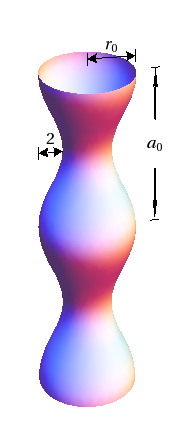
For this development, we will use a parametrized surface given by
\begin{equation*}
\vr(s,t) = x(s,t) \vi + y(s,t) \vj + z(s,t) \vk
\end{equation*}
with \(a \leq s \leq b\) and \(c \leq t \leq d\text{.}\) Although we illustrate the idea using a rectangular domain in the \(st\)-plane, this same approach works for non-rectangular domains. The partial derivatives of this parameterization
\begin{align*}
\vr_s(s,t) \amp = x_s(s,t) \vi + y_s(s,t) \vj + z_s(s,t) \vk\\
\vr_t(s,t) \amp = x_t(s,t) \vi + y_t(s,t) \vj + z_t(s,t) \vk
\end{align*}
give vectors tangent to the surface in the direction of change in \(s\) and \(t\text{,}\) respectively.
To break the section of the surface into steps in
\(s\) and
\(t\text{,}\) we partition the interval of
\(s\)-values
\([a,b]\) into
\(m\) subintervals of length
\(\Delta s = \frac{b-a}{m}\) and let
\(s_0\text{,}\) \(s_1\text{,}\) \(\ldots\text{,}\) \(s_m\) be the endpoints of these subintervals, where
\(a = s_0\lt s_1\lt s_2 \lt \cdots \lt s_m = b\text{.}\) We also partition the interval of
\(t\)-values
\([c,d]\) into
\(n\) subintervals of equal length
\(\Delta t = \frac{d-c}{n}\) and let
\(t_0\text{,}\) \(t_1\text{,}\) \(\ldots\text{,}\) \(t_n\) be the endpoints of these subintervals, where
\(c = t_0\lt t_1\lt t_2 \lt \cdots \lt t_n = d\text{.}\)
These subintervals partition the rectangle
\(R\) with
\(a\leq s\leq b\) and
\(c\leq t\leq d\) in
\(st\)-coordinates into
\(mn\) sub-rectangles
\(R_{ij}\) with opposite vertices
\((s_{i-1},t_{j-1})\) and
\((s_i, t_j)\) for
\(i\) between
\(1\) and
\(m\) and
\(j\) between
\(1\) and
\(n\text{.}\) These rectangles all have equal area
\(\Delta A = \Delta s \cdot \Delta t\text{.}\)
Each of these rectangles from the
\(st\)-domain splits the surface into an
\(m\times n\) grid of patches, but these patches of the surface do
not all have the same (surface) area.
Figure 13.10.9 shows a surface with traces given for five equally-spaced values of
\(s\) and
\(t\text{.}\) This breaks the surface into a
\(4\times 4\) grid of patches. Since these patches of the surface do not have the same surface area, we estimate the surface area for each particular piece of the grid using the tools from the parameterization.
Each of the pieces of the surface corresponds to increasing
\(s\) by a small amount
\(\Delta s\) or increasing
\(t\) by a small amount
\(\Delta t\) from the point
\((s_{i-1},t_{j-1})\) in the
\(st\)-parameter plane. We want to find the vectors corresponding to each of the sides of the orange parallelogram in
Figure 13.10.9. In particular, the vector
\(\vr_t \Delta t\) corresponds to the side of the parallelogram along a constant value of
\(s\) (shown as a yellow vector in
Figure 13.10.9) and
\(\vr_s \Delta s\) corresponds to the side of the parallelogram along a constant value of
\(t\) (shown as a red vector in
Figure 13.10.9).
The area of this parallelogram is \(S_{ij}=\vecmag{(\vr_s \Delta s) \times (\vr_t \Delta t)}\) evaluated at the point \((s_{i-1},t_{j-1})\text{.}\) This is an approximation of the surface area for a patch of the surface. The magnitude simplifies to \(S_{ij}=\vecmag{\vr_s \times \vr_t} \Delta s \Delta t\text{,}\) which means that the approximation over all of these pieces of the grid sums to
\begin{equation}
SA\approx \sum_{i=1}^m \sum_{j=1}^n S_{ij}= \sum_{i=1}^m \sum_{j=1}^n \vecmag{\vr_s(s_{i-1},t_{j-1}) \times \vr_t(s_{i-1},t_{j-1})} \Delta s \Delta t\text{.}\tag{13.10.3}
\end{equation}
We have now completed both the first and second steps of the classic calculus approach by approximating the surface area and quantifying how the approximation changes with a smaller scale of steps (in
\(s\) and
\(t\)). You can use
Figure 13.10.12 to see how increasing the number of pieces gives successively better approximations for the surface area of each piece.
Note that this approximation is a double Riemann sum corresponding to a double integral. In particular, taking the limit as
\(\Delta s\) and
\(\Delta t\) go to zero, the Riemann sum becomes a double integral of
\(\vecmag{\vr_s \times \vr_t}\) over the rectangular region of integration with
\(a \leq s \leq b\) and
\(c \leq t \leq d\text{,}\) which gives the following formula for calculating the surface area.