Given a function \(f\) of the variables \(x\) and \(y\text{,}\) what does the rate of change with respect to either \(x\) or \(y\) tell us about the graph of \(z=f(x,y)\text{?}\)
This section heavily relies on students to understand traces as the intersection of the surface plot of \(z=f(x,y)\) with a fundamental plane which allows us to simplify our multivariable problems into a single variable problem where we have lots of experience. This section also relates first partial derivatives to properties of multivariable functions on surface plots, contour plots, and tables. This section can be covered in a single class meeting but some instructors will pair this section with Section 11.5 to talk about partial derivatives as a unified concept.
The last several activities offer a variety of applications and related approximation ideas for first partial derivatives. You may want to pick one of these and assign others as exercises.
The derivative plays a central role in single-variable calculus because it provides important information about a function in terms of each of the representations of the function. Thinking graphically, the derivative at a point tells us the slope of the line tangent to the graph at the given point. Numerically, the derivative at a point also provides the instantaneous rate of change of the function with respect to a change in the input variable. Algebraically, we can calculate the derivative as a function of the same input variable, which is useful as a tool to examine where the function is increasing or decreasing, as well as the concavity of the function’s graph.
In this chapter, we are investigating functions of two or more variables and we can still ask how fast a function of several variables is changing, but we have to be careful about what we mean. Thinking graphically again, we can try to measure how steep the graph of the function is in a particular direction. As we saw in Section 11.3, the idea of measuring the behavior of a two variable function in a particular direction and generalizing to other directions is a much deeper idea when considering multiple input variables. Alternatively, we may want to know how quickly a function’s output is changing in response to varying only one of the inputs. Over the next few sections, we will develop tools for addressing these questions. We begin with a Preview Activity that considers how we can apply our knowledge of single-variable calculus to measure the rate of change when we hold all but one input variable constant.
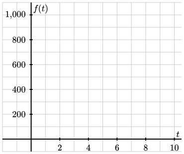
Suppose the interest rate on loans is fixed at \(3\%\text{.}\) Express \(M\) as a function \(f\) of \(t\) alone using \(r=0.03\text{.}\) That is, let \(f(t) = M(0.03, t)\text{.}\) Sketch the graph of \(f\) on the axes below and write a couple of sentences to explain the meaning of the function \(f\text{.}\)
Axes for sketching the graph of \(f(t)\text{.}\) The horizontal axis shows \(t\)-values from 0 to 10 and the vertical axis shows \(f(t)\) values from 0 to 1000.
Find the instantaneous rate of change \(f'(4)\) and state the units on this quantity. What information does \(f'(4)\) tell us about our car loan? What information does \(f'(4)\) tell us about the graph you sketched in (b)?
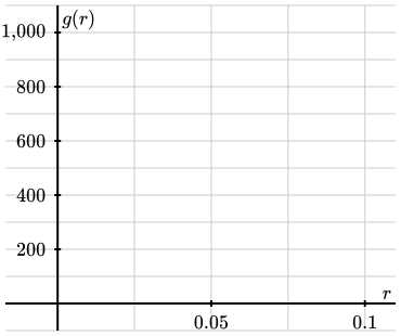
Suppose that we want to examine how the monthly payment will change if we plan to take 4 years to pay off the loan. Express \(M\) as a function of the interest rate \(r\) with a fixed loan term of \(t=4\text{.}\) That is, let \(g(r) = M(r, 4)\text{.}\) Give the function \(g(r)\) and sketch a graph of \(g\) on the axes provided. Write a couple of sentences to explain the meaning of the function \(g\text{.}\)
Axes for sketching the graph of \(g(r)\text{.}\) The horizontal axis shows \(r\)-values from 0 to 0.10 and the vertical axis shows \(g(r)\) values from 0 to 1000.
Find the instantaneous rate of change \(g'(0.03)\) and state the units on this quantity. Write a couple of sentences to explain what \(g'(0.03)\) tell us about the car loan. What information does \(g'(0.03)\) tell us about the graph you sketched in (d)?
In Section 11.2, we studied the behavior of a function of two or more variables by considering the traces of the function. By holding one of our input variables constant, we restricted our multivariable function to have only one input variable, which means we can use all of our calculus tools from single-variable calculus on these traces.
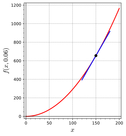
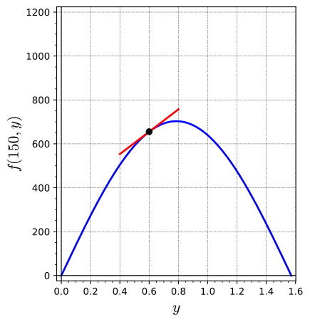
This function measures horizontal distance (in feet) traveled by a projectile launched with an initial speed of \(x\) feet per second at an angle of \(y\) radians to the horizontal. The graph of this function is shown in Figure 11.4.1 with traces plotted on the surface for \(x=150\) (in blue) and \(y=0.6\) (in red).
A three dimensional plot of a curved surface that this is u-shaped along constant values of one coordinate and increases parabolically as that the other horizontal coordinate is increased. On the lower corner of this curved surface are drawn three mutually perpendicular line segments labeled \(x\text{,}\)\(y\text{,}\) and \(z\) signifying origin. In the direction of the segment labeled y from the origin, there is a two dimensional flat grid labeled \(x\) horizontally and \(z\) vertically. A branch of a parabola is shown in red from the bottom left of this grid to the top right. This red curve is copied along the curved surface along a direction that is parallel to the segment labeled x (from the origin). In the direction of the segment labeled x from the origin, there is a two dimensional flat grid labeled \(y\) horizontally and \(z\) vertically. A parabola is shown in blue pointing downward on this grid with a vertex about half way up the grid. This blue curve is copied along the curved surface along a direction that is parallel to the segment labeled y (from the origin).
A two dimensional plot with the horizontal axis labeled \(x\) going from 0 to 200. The vertical axis is labeled \(f(x,0.06)\) and goes from 0 to 1200. An upward facing parabola is drawn in red from (0,0) to (200,1150). A point on the parabola at (150,750) is drawn in black and a line segment tangent to the red parabola at the highlighted point is drawn in blue.
Since the trace is a function of only one variable, we can consider its derivative exactly as we did in single-variable calculus. With \(y=0.6\text{,}\) we have
Thinking of this derivative as an instantaneous rate of change implies that for a fixed launch angle of \(0.6\) radians, increasing the initial speed of the projectile by one foot per second leads to an expected increase in the horizontal distance traveled of approximately 8.74 feet. Since the sign of the derivative of the trace is positive there would be an increase to the range of the projectile if we increased the initial speed from \(150\, \text{ft/s}\) while holding the launch angle constant at \(0.6\) radians.
By holding \(y\) fixed and differentiating with respect to \(x\text{,}\) we obtain the first-order partial derivative of \(f\) with respect to \(x\). Denoting this partial derivative as \(f_x\text{,}\) we have seen that
A two dimensional plot with the horizontal axis labeled \(y\) going from 0 to 1.6. The vertical axis is labeled \(f(150,y)\) and goes from 0 to 1200. An downward facing parabola is drawn in blue with vertex at \((\frac{\pi}{4},700)\text{.}\) A point on the parabola at (0.6,650) is drawn in black and a line segment going up and to the right, tangent to the blue parabola at the highlighted point, is drawn in red.
Once again, the derivative gives the slope of the tangent line shown on the right in Figure 11.4.3. Thinking of this derivative as an instantaneous rate of change, we expect that, for a fixed initial speed of the projectile of 150 feet per second, the range of the projectile increases by approximately 509.5 feet for every radian we increase the launch angle \(y\text{.}\)
By holding \(x\) fixed and differentiating with respect to \(y\text{,}\) we obtain the first-order partial derivative of \(f\) with respect to \(y\). As before, we denote this partial derivative as \(f_y\) and write
As with the partial derivative with respect to \(x\text{,}\) we may express this quantity more generally at an arbitrary point \((a,b)\text{.}\) To recap, we have now arrived at the formal definition of the first-order partial derivatives of a function of two variables.
We did not use the classic calculus approach in our development here because we defined the partial derivatives along a trace of our function, which restricts our function to one variable. As you will see in the next several activities, this allows us to continue using ideas from single variable calculus rather than needing to develop new multivariable tools.
In this activity, we will be examining the function \(\displaystyle f(x,y) = \frac{x y^2}{x+1}\) at the point \((1,2)\text{.}\) Specifically, we will be looking at how the traces of this function will be related to the values of the partial derivatives.
Write a formula for the trace \(f(x,2)\) as a function of \(x\text{.}\) On the axes provided, draw the graph of the trace with \(y=2\) around the point where \(x=1\text{.}\) Then sketch the tangent line at the point with \(x=1\) on your graph.
Write a formula for the trace \(f(1,y)\) as a function of \(y\text{.}\) On the axes provided, draw the graph of the trace with \(x=1\text{.}\) Then sketch the tangent line at the point with \(y=2\) on your graph.
What we have seen so far demonstrates that each partial derivative at a point arises as the derivative of a function of one variable defined by fixing all other coordinates. 1
At this stage, we have considered partial derivatives for functions of two variables, but the methods generalize to functions of three or more variables by fixing all but one variable.
In addition, we may consider each partial derivative as defining a new function with input given by the point \((x,y)\text{,}\) just as the derivative \(f'(x)\) defines a new function of \(x\) in single-variable calculus. Due to the connection between single-variable derivatives and partial derivatives, we often use Leibniz-style notation to denote partial derivatives by writing
\begin{equation*}
\frac{\partial f}{\partial x}(a, b) = f_x(a,b),
\
\mbox{and}
\
\frac{\partial f}{\partial y}(a, b) = f_y(a,b)\text{.}
\end{equation*}
We read the notation \(\partial f/\partial x\) as “partial \(f\)-partial \(x\)”.
To calculate the partial derivative \(f_x\text{,}\) we hold \(y\) fixed. In other words, we treat \(y\) as a constant. In Leibniz notation, observe that
To see the contrast between how we calculate single-variable derivatives and partial derivatives and the difference between the notations \(\frac{d}{dx}\bigl[ \ \bigr]\) and \(\frac{\partial}{\partial x}\bigl[ \ \bigr]\text{,}\) observe that
Because there is a lot going on in the computations above, let us highlight some terms for emphasis. Note that when we are interested in computing the partial derivative with respect to \(x\) of a term of the form \(x^2y\text{,}\) we can factor out the \(y\) as if it were a coefficient because \(y\) is constant with respect to changes in \(x\). Algebraically, this can be expressed as
Similarly, when we are computing the partial derivative with respect to \(x\) of a term of the form \(2y\text{,}\) the entire term is constant with respect to \(x\text{.}\) Thus,
To summarize, computing partial derivatives can be done directly by applying familiar differentiation rules from single-variable calculus, but we do so while holding all but one of the variables constant. The next activity has you practice computing partial derivatives using these ideas.
Subsection11.4.3Interpreting and Estimating First-Order Partial Derivatives
Throughout single-variable calculus, you frequently used the fact that the derivative of a single-variable function can be interpreted geometrically as the slope of the line tangent to the graph at a given point. Similarly, we have seen that the partial derivatives measure the slope of a line tangent to a trace of a function of two variables as shown in Figure 11.4.5. Use the drop-down to change the trace and tangent line shown or show both traces and tangent lines.
An interactive three dimensional plot with three axes labeled \(x\) and \(y\) horizontally and \(z\) vertically. A surface is shown in gray with a grid of lines along the surface. The surface is shown for a patch above the first quadrant and the surface increases vertically as either \(x\) or \(y\) decreases. A dropdown option at the top of the figure allows for three options. The “x-trace only” plots a plane in red that is parallel to the yz-plane, is labeled \(y=b\text{,}\) and highlights the curve along the surface and on the red plane in red. The “y-trace only” plots a plane in blue that is parallel to the xz-plane, is labeled \(x=a\text{,}\) and highlights the curve along the surface and on the blue plane in blue. The “both traces” option shows both of the plots described above.
Beyond representing the slope of the tangent line to the graph of a one-variable function or to a trace of a multivariable function, the values of derivatives and partial derivatives at a point give us the instantaneous rate of change of the function at that point. This perspective makes it possible for us to contemplate the units on partial derivatives, as the next activity asks you to investigate.
The speed of sound \(C\) traveling through ocean water is a function of temperature, salinity and depth. It may be modeled by the function
\begin{align*}
C \amp= 1449.2+4.6T-0.055T^2+0.00029T^3 \\
\amp \quad +(1.34-0.01T)(S-35)+0.016D \text{.}
\end{align*}
Here \(C\) is the speed of sound in meters/second, \(T\) is the temperature in degrees Celsius, \(S\) is the salinity in grams/liter of water, and \(D\) is the depth below the ocean surface in meters.
State the units for each of the partial derivatives, \(C_T\text{,}\)\(C_S\) and \(C_D\text{.}\) For each partial derivative, write a sentence that explains the physical meaning of the partial derivatives in terms of the rate of change for \(C\text{.}\)
Evaluate each of the three partial derivatives at the point where \(T=10\text{,}\)\(S=35\) and \(D=100\text{.}\) Write a few sentences to explain what the sign of each partial derivatives tell us about the behavior of the function \(C\) at the point \((10,35, 100)\text{.}\)
In single-variable calculus, you considered not only functions represented algebraically, but also those represented using tables of data or graphs. You used these representations and the difference quotient \(\frac{f(a+h)-f(a)}{h}\) to estimate derivatives. This is possible because for a function \(f\) of a single variable \(x\) at a point where \(x=a\text{,}\) the difference quotient tells us the average rate of change of \(f\) over the interval \([a,a+h]\text{,}\) while the derivative \(f'(a)\) tells us the instantaneous rate of change of \(f\) at \(x=a\text{.}\) We can use a similar relationship between limits of difference quotients and partial derivatives to provide context and meaning to partial derivatives as a measurement. To do this, we need to make sure we are holding all but one input variable constant when we compute the difference quotient. The next two activities are focused on the meaning of partial derivatives using a table as a numerical representation of a multivariable function (Activity 11.4.5) and using a contour plot as a graphical representation of a multivariable function (Activity 11.4.6).
The wind chill, as frequently reported, is a measure of how cold it feels outside when the wind is blowing. In the table below, the wind chill \(w\) is a function of the wind speed \(v\) and the ambient air temperature \(T\text{.}\) Both \(w\) and \(T\) are measured in degrees Fahrenheit, while \(v\) is measured in miles per hour. This means that \(w\) can be expressed in the form \(w = w(v, T)\text{.}\)
When computing the partial derivative with respect to wind speed \(w_v\text{,}\) which variable is held constant and which variable changes? Do you think \(w_v\) is positive, negative, or zero at \((v,T)=(20,-10)\text{?}\) Write a couple of sentences to explain your reasoning.
When computing the partial derivative with respect to temperature \(w_T\text{,}\) which variable is held constant and which variable changes? Do you think \(w_T\) is positive, negative, or zero at \((v,T)=(20,-10)\text{?}\) Write a couple of sentences to explain your reasoning.
Recall that we can estimate a partial derivative of a single variable function \(f\) using the central difference \(\frac{f(x+h)-f(x-h)}{2h}\) for small values of \(h\text{.}\) A partial derivative is a derivative of an appropriate trace, so by considering a difference quotient for a trace of \(w\text{,}\) estimate the partial derivative \(w_v(20,-10)\text{.}\) Include units on your answer and write a sentence explaining the meaning of the value of \(w_v(20,-10)\text{.}\)
Recall from single-variable calculus that for a function \(f\text{,}\)\(f(a+h) \approx f(a) + hf'(a)\text{.}\) Use this idea and your result above to estimate the wind chill \(w(18, -10)\text{.}\)
Estimate the partial derivative \(w_T(20,-10)\text{.}\) Include units on your answer and write a sentence explaining the meaning of the value of \(w_T(20,-10)\text{.}\)
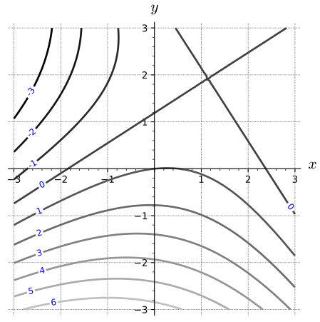
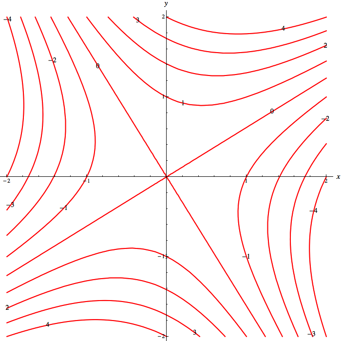
Shown below is a contour plot of a function \(f\text{.}\) The output values of the function are indicated on the contours. This activity will ask you to use this contour plot to estimate some partial derivatives of \(f\text{.}\)
A two dimensional plot with horizontal coordinate labeled \(x\) going from -3 to 3 and vertical coordinate labeled \(y\) going from -3 to 3. A pair of intersecting lines with positive and negative slopes from a point near (1,2) are labeled 0. Hyperbolic curves are with the intersecting lines as asymptotes. The hyperbolic curves below these intersecting lines are labeled from 1 to 6 as they move away from (1,2). The curves going to the left from (1,2) are labeled from -1 to -3.
When computing \(f_x\text{,}\) which variable is treated as a constant? On the contour plot, sketch a line segment for which that variable is constant through the point \((-2,-1)\) .
To estimate \(f_x(-2,-1)\) using a difference quotient, you must identify two points in the \(xy\)-plane that are near \((-2,-1)\text{,}\) on the line segment you sketched in the previous part (or an extension of that line segment), and for which you can use the contour plot to find the value of the function at those points. Mark these points, which we will call \((a_1,b_1)\) and \((a_2,b_2)\) on your contour plot and record the values of \(f\) at these points.
If possible, you will use a central difference, but if your points are not equally spaced from \((-2,-1)\text{,}\) you may have a different expression that is still a difference quotient.
In this part and the next, you will need to follow a similar process to the previous part. However, the activity does not break down the steps each time. Estimate the partial derivative \(f_y(-2,-1)\text{.}\)
Notice that the approximations, algebraic rules, and interpretations developed in this section for partial derivatives are the same as in single-variable calculus. Additionally, the form of the difference quotients and limit definition for partial derivatives maintains the same form as in single-variable calculus, which we also saw when studying vector-valued functions of one variable in the previous chapter:
\begin{equation*}
\text{rate of change}= \lim \frac{\text{change in output of function}}{\text{change in input of function}}
\end{equation*}
Importantly and conveniently, all of the change we look at with a partial derivative is with respect to a single input variable as we consider holding all other input variables constant.
Notice that in this section, we did not need to use the classic calculus approach from scratch to define the partial derivative because we restricted our multivariable function along a trace to be a single-variable function. This was convenient, but we will soon see that we will need new tools to make similar arguments when studying the rate of change of a multivariable function in a direction that is not along a trace such as \(x=a\) or \(y=b\text{.}\)
If \(f=f(x,y)\) is a function of two variables, there are two first-order partial derivatives of \(f\text{:}\) the partial derivative of \(f\) with respect to \(x\text{,}\)
The partial derivative \(f_x(a,b)\) tells us the instantaneous rate of change of \(f\) with respect to \(x\) at \((x,y) = (a,b)\) when \(y\) is fixed at \(b\text{.}\) Geometrically, the partial derivative \(f_x(a,b)\) tells us the slope of the line tangent to the \(y=b\) trace of the function \(f\) at the point \((a,b,f(a,b))\text{.}\)
The partial derivative \(f_y(a,b)\) tells us the instantaneous rate of change of \(f\) with respect to \(y\) at \((x,y) = (a,b)\) when \(x\) is fixed at \(a\text{.}\) Geometrically, the partial derivative \(f_y(a,b)\) tells us the slope of the line tangent to the \(x=a\) trace of the function \(f\) at the point \((a,b,f(a,b))\text{.}\)
Suppose that \(f(x,y)\) is a smooth function and that its partial derivatives have the values, \(f_x(3, -9) = 3\) and \(f_y(3, -9) =
1\text{.}\) Given that \(f(3, -9) = -1\text{,}\) use this information to estimate the value of \(f(4, -8)\text{.}\) Note this is analogous to finding the tangent line approximation to a function of one variable. In fancy terms, it is the first Taylor approximation.
The gas law for a fixed mass \(m\) of an ideal gas at absolute temperature \(T\text{,}\) pressure \(P\text{,}\) and volume \(V\) is \(PV = mRT\text{,}\) where \(R\) is the gas constant.
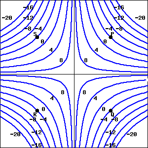
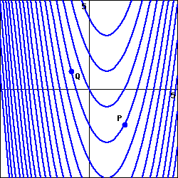
Determine the sign of \(f_x\) and \(f_y\) at each indicated point using the contour diagram of \(f\) shown below. (The point \(P\) is that in the first quadrant, at a positive \(x\) and \(y\) value; \(Q\) through \(T\) are located clockwise from \(P\text{,}\) so that \(Q\) is at a positive \(x\) value and negative \(y\text{,}\) etc.)
A plot of circles centered at the origin. The smallest circle is labeled 6 and successively larger circles are labeled 9, 12, 15,18,21, 24. The difference in radius between successive circles is decreasing. A point labeled P is on the contour labeled 12 and in the first quadrant. A point labeled Q is on the contour labeled 12 and is in the fourth quadrant. A point labeled S is on the contour labeled 12 and in the second quadrant. A point labeled R is on the contour labeled 12 and is in the third quadrant.
An experiment to measure the toxicity of formaldehyde yielded the data in the table below. The values show the percent, \(P=f(t,c)\text{,}\) of rats surviving an exposure to formaldehyde at a concentration of \(c\) (in parts per million, ppm) after \(t\) months.
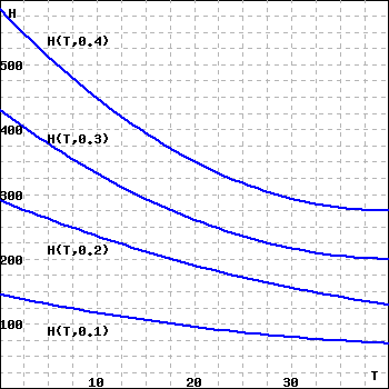
An airport can be cleared of fog by heating the air. The amount of heat required depends on the air temperature and the wetness of the fog. The figure below shows the heat \(H(T,w)\) required (in calories per cubic meter of fog) as a function of the temperature \(T\) (in degrees Celsius) and the water content \(w\) (in grams per cubic meter of fog). Note that this figure is not a contour diagram, but shows cross-sections of \(H\) with \(w\) fixed at \(0.1\text{,}\)\(0.2\text{,}\)\(0.3\text{,}\) and \(0.4\text{.}\)
A graph showing \(H(T,0.1), H(T,0.2), H(T,0.3), H(T,0.4)\text{,}\) which are decreasing functions of \(T\text{,}\) each at a higher value of \(H\text{.}\) As \(H\) increases, the associated level curve is more concave up.
The following questions refer to the table shown below, giving the temperature adjusted for wind-chill, \(C\text{,}\) in \({}^\circ\) F, as a function \(f(w,T)\) of the wind speed, \(w\text{,}\) in mph, and the temperature, \(T\text{,}\) in \({}^\circ\) F. The temperature adjusted for wind-chill tells you how cold it feels, as a result of the combination of wind and temperature.
\(0\le x\le 1\text{.}\) On a sheet of paper, sketch a graph of \(H\) against \(x\) for \(t=0\) and \(t=1\text{.}\) Think about why your graphs make sense.
(Be sure that you can say in words what the practical interpretation (in terms of temperature) of these two partial derivatives is, and why each has the sign that it does.)
The Heat Index, \(I\text{,}\) (measured in apparent degrees F) is a function of the actual temperature \(T\) outside (in degrees F) and the relative humidity \(H\) (measured as a percentage). A portion of the table which gives values for this function, \(I=I(T,H)\text{,}\) is reproduced in Table 11.4.6.
State the limit definition of the value \(I_T(94,75)\text{.}\) Then, estimate \(I_T(94,75)\text{,}\) and write one complete sentence that carefully explains the meaning of this value, including its units.
State the limit definition of the value \(I_H(94,75)\text{.}\) Then, estimate \(I_H(94,75)\text{,}\) and write one complete sentence that carefully explains the meaning of this value, including its units.
Suppose you are given that \(I_T(92,80) = 3.75\) and \(I_H(92,80) = 0.8\text{.}\) Estimate the values of \(I(91,80)\) and \(I(92,78)\text{.}\) Explain how the partial derivatives are relevant to your thinking.
On a certain day, at 1 p.m. the temperature is 92 degrees and the relative humidity is 85%. At 3 p.m., the temperature is 96 degrees and the relative humidity 75%. What is the average rate of change of the heat index over this time period, and what are the units on your answer? Write a sentence to explain your thinking.
Let \(f(x,y) = \frac{1}{2}xy^2\) represent the kinetic energy in Joules of an object of mass \(x\) in kilograms with velocity \(y\) in meters per second. Let \((a,b)\) be the point \((4,5)\) in the domain of \(f\text{.}\)
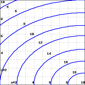
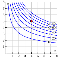
Often we are given certain graphical information about a function instead of a rule. We can use that information to approximate partial derivatives. For example, suppose that we are given a contour plot of the kinetic energy function (as in Figure 11.4.7) instead of a formula. Use this contour plot to approximate \(f_x(4,5)\) and \(f_y(4,5)\) as best you can. Compare to your calculations from earlier parts of this exercise.
Assume that temperature is measured in degrees Celsius and that \(x\) and \(y\) are each measured in inches. (Note: At no point in the following questions should you expand the denominator of \(C(x,y)\text{.}\))
If an ant is on the metal plate, standing at the point \((2,3)\text{,}\) and starts walking in the direction parallel to the positive \(y\) axis, at what rate will the temperature the ant is experiencing change? Explain, and include appropriate units.
If an ant is walking along the line \(y = 3\) in the positive \(x\) direction, at what instantaneous rate will the temperature the ant is experiencing change when the ant passes the point \((1,3)\text{?}\)
Now suppose the ant is stationed at the point \((6,3)\) and walks in a straight line towards the point \((2,0)\text{.}\) Determine the average rate of change in temperature (per unit distance traveled) the ant encounters in moving between these two points. Explain your reasoning carefully. What are the units on your answer?
Determine the equation of the plane that passes through the point \((2,1,f(2,1))\) whose normal vector is orthogonal to the direction vectors of the two lines found in (b) and (c).
Use a graphing utility to plot both the surface \(z = 8 - x^2 - 3y^2\) and the plane from (e) near the point \((2,1)\text{.}\) What is the relationship between the surface and the plane?
Recall from single variable calculus that, given the derivative of a single variable function and an initial condition, we can integrate to find the original function. We can sometimes use the same process for functions of more than one variable. For example, suppose that a function \(f\) satisfies \(f_x(x,y) = \cos(y)e^x+2x+y^2\text{,}\)\(f_y(x,y) = -\sin(y)e^x+2xy+3\text{,}\) and \(f(0,0) = 5\text{.}\)
Find all possible functions \(f\) of \(x\) and \(y\) such that \(f_x(x,y) = \cos(y)e^x+2x+y^2\text{.}\) Your function will have both \(x\) and \(y\) as independent variables and may also contain summands that are functions of \(y\) alone.