What geometric condition enables us to optimize a function \(f=f(x,y)\) subject to a constraint given by \(g(x,y) = k\text{,}\) where \(k\) is a constant?
This section requires the optimization tools from Section 11.10 and the interpretations of the gradient from Section 11.8 and Section 11.9. This section is omitted for time by some instructors but a requirement at some institutions with engineering programs that need this topic covered. This section can likely be covered in a single class, but that depends a lot on students’ algebraic proficiency, as the nonlinear systems that arise in these problems can be challenging for students. Students tend to find the fact that there is not one method that will solve all of these systems frustrating, so giving them a variety of problems to practice on is important for instructors who will be giving anything but the most routine Lagrange multiplier problem on an exam. We have placed the geometric aspect (parallel gradients) prominently throughout the section, which allows for asking graphical questions that do not require intensive algebra questions a viable conceptual method for testing students on this material.
We previously considered how to find the extreme values of functions on both unrestricted domains and closed, bounded domains. Other types of optimization problems involve maximizing or minimizing a quantity subject to an external constraint. In these cases the extreme values frequently won’t occur at the points where the gradient is zero, but rather at other points that satisfy an important geometric condition. These problems are called constrained optimization problems and can be solved with the method of Lagrange Multipliers, which we study in this section. This method also provides an alternative approach to looking for maxima or minima on the boundary of a closed, bounded domain and can be useful in cases where parameterizing the boundary is more difficult than the situation we saw in Example 11.10.13.
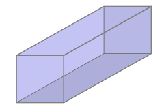
A shipping company places a restriction on packages so that the sum of the package’s length and girth must be at most 12 feet. (The girth is the perimeter of the smallest end of the package.) Our goal is to find the largest possible volume of a rectangular package with a square end that can be sent by this shipping company.
Let \(x\) be the length in feet of the side of one square end of the package and \(y\) be the length in feet of the package. This allows us to define a function that gives the volume of the package as \(f(x,y) = x^2y\) cubic feet. The girth of the package is \(4x\text{,}\) so we can define \(g(x,y)=4x+y\) to be the sum of the girth and length. The domain on which we wish to maximize \(f\) is all points for which \(x\geq 0\text{,}\)\(y\geq 0\text{,}\) and \(g(x,y)\leq 12\text{.}\) A moment of reflection should confirm that any package with \(g(x,y)\lt 12\) cannot maximize the volume, as increasing either \(x\) or \(y\) so that \(g(x,y)\) remains at most 12 will only lead to a larger volume.
Thus, we say that we wish to maximize \(f(x,y) = x^2y\) subject to the constraint \(g(x,y) = 4x+y = 12\text{.}\) We call \(f\) the objective function since it is our goal to find extreme values for this function. We call \(g\) our contraint function because we are constrainted (limited) to a specific value of this function.
Compute \(\nabla f\) and evaluate the gradient at the points \(P_1:(1,8)\text{,}\)\(P_2:(1.5,6)\text{,}\)\(P_3:(2,4)\text{,}\) and \(P_4:(2.5,2)\text{.}\)
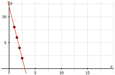
The plot below shows the graph of \(g(x) = 12\) as well as the four points for which you evaluated \(\nabla f\) in the previous part. Sketch \(\nabla f\) at each of the four points. You may not have enough space to sketch get the magnitude of each gradient vector correct, but you should accurately depict the direction of each of the four vectors.
Coordinate axes for the \(xy\)-plane along with a line passing through the points \((12,0)\) and \((3,0)\text{.}\) On the line, four points are marked. These points are \((1,8)\text{,}\)\((1.5,6)\text{,}\)\((2,4)\text{,}\) and \((2.5,2)\text{.}\) The vectors all point to the right of the line. The vectors emanating from \((1,8)\) and \((1.5,6)\) both below and right of the perpendicular to the given line. The vector emanating from \((2.5,2)\) points above and right of the perpendicular to the given line. The vector emanating from \((2,4)\) is perpendicular to the given line.
Compute \(\grad g\text{.}\) Describe the geometric relationship between \(\nabla g\) and the line \(g(x,y) = 12\) plotted in the previous part and why they have this relationship.
Recall that the gradient always points in the direction of steepest ascent. However, in this constrained optimization setting, the domain that we allowed to consider for \(f\) is only those points for which \(g(x,y)=12\text{.}\) Thus, we may not be able to move in the direction of the gradient while staying within the domain. Look back at the four points at which you sketched \(\nabla f\) in part (b). For each point, identify which direction you could move along the line to increase the value of \(f\text{.}\) What is the relationship between \(\nabla f\) and \(\nabla g\) at a point where you cannot move along the line while increasing the value of \(f\text{?}\)
Subsection11.11.2Constrained Optimization and Lagrange Multipliers
We will further examine our work in Preview Activity 11.11.1 to motivate and understand the general method for solving constrained optimization problems. In Preview Activity 11.11.1, we considered an optimization problem where there is an external constraint on the variables, namely that the girth plus the length of the package cannot exceed 12 feet.
You saw in your plots that the direction to move in the \((x,y)\)-plane to increase the volume would take you off of the constraint line. For points \(P_1\) and \(P_2\) you saw how moving down on the constraint line would move you at least a little bit in the direction of greatest increase (as measured by \(\nabla f\)). Similarly, at points \(P_3\) and \(P_4\) you could move up the constraint line to increase the value of the objective function. So somewhere between \(P_2\) and \(P_3\) there has to be a place where moving down the constraint line will no longer increase the output of our objective function.
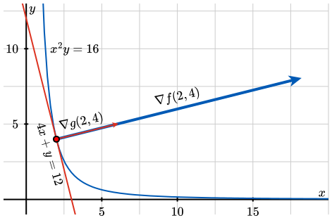
Ultimately, we observed that the gradient of the objective function \(f\) and the gradient of the constraint \(g\) must be parallel when we maximize \(f\) subject to the constraint. This is because the only way to increase the value of the objective function at such a point is to move off of the constraint curve, which is not allowed. In Figure 11.11.2, we show the contour \(f(x,y)=x^2y = 16\text{,}\) the constraint \(g(x,y) = 4x+y=12\text{,}\) and the point \((2,4)\) at which these two intersect. We have also included the gradients at this point, illustrating that the gradients are parallel.
A hyperbola labeled \(x^2y=16\) in the first quadrant. The line \(4x+y=12\) is also shown. The line is tangent to the hyperbola at \((2,4)\text{.}\) This point is the tail of two parallel vectors, which are labeled \(\nabla g(2,4)\) and \(\nabla f(2,4)\text{.}\) The gradient of \(f\) is the longer vector.
After doing the preview activity and looking at Figure 11.11.2, you may be wondering if there are other contours that intersect the constraint line and have a point where the gradient to the objective function and the gradient to the constraint function are parallel. In the next example, we will set up an algebraic approach to finding all points on the constraint where the gradients of the objective and constraint functions are parallel and then find where maximum and minimum values occur for the objective function.
Now recall that two vectors are parallel exactly when one is a scalar multiple of the other. Algebraically, this happens when one vector is a scalar multiple of the other:
\begin{equation}
\nabla f = \lambda g\text{.}\tag{11.11.1}
\end{equation}
We refer to the scalar \(\lambda\) as a Lagrange multiplier. For our objective and constraint functions, this gives rise to the system of equations:
Now we must solve the system of equations to find all points where the gradients of \(f\) and \(g\) will be parallel. We can use (11.11.3) to give us an expression for \(\lambda\) that can be substituted into (11.11.2). This gives the equation \(2xy = 4x^2\text{,}\) which is equivalent to
From this, we can see that either \(x=0\) or \(y=2x\text{.}\) It is important that we not “cancel” the \(x\) from \(2xy = 4x^2\text{,}\) as that would lead to us losing the solution \(x=0\text{.}\) We can now substitute these solutions into (11.11.4), which gives us \(y=12\) when \(x=0\) and \(4x+2x=12\) or \(x=2\) when \(y=2x\text{.}\) Substituting \(x=2\) into (11.11.4) gives us \(y=4\text{.}\) Thus we need to consider the points \((0,12)\) and \((2,4)\text{.}\)
Conceptually, the point \((0,12)\) would correspond to a minimum volume of zero because the side length on the square side of our box would be zero. Algebraically, we get \(f(0,12)=0\text{.}\) On the other hand, \(f(2,4) = 16\text{,}\) so we have a maximum value of 16 cubic feet for a rectangular package with a square end subject to the given constraint. You should note that this point occurs between \(P_2\) and \(P_3\text{,}\) as we previously reasoned.
The general technique for optimizing a function \(f = f(x,y)\) subject to a constraint \(g(x,y)=c\) is to solve the system \(\nabla f = \lambda \nabla g\) and \(g(x,y)=c\) for \(x\text{,}\)\(y\text{,}\) and \(\lambda\text{.}\) We then evaluate the function \(f\) at each point \((x,y)\) that results from a solution to the system in order to find the optimum values of \(f\) subject to the constraint.
Before getting a chance to practice with the algebraic aspects of Lagrange multipliers, the next activity gives you a chance to review your geometric understanding of the method.
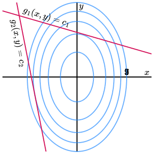
Below is the contour plot of a function \(f(x,y)\text{.}\) Also shown are two lines, which are constraint curves. Use the plot to identify the extreme value(s) of \(f(x,y)\) subject to the constraint \(g_1(x,y)=c_1\) and the point(s) at which these extrema occur. Repeat this for the constraint \(g_2(x,y)=c_2\text{.}\) Write a sentence to explain your reasoning.
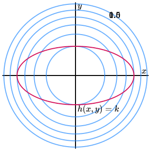
The circular curves in the graph below are contours of a function \(T(x,y)\text{.}\) Use the plot to identify the extreme value(s) of \(T(x,y)\) subject to the constraint \(h(x,y)=k\text{,}\) which is also shown in the plot. Also identify the points at which the extreme value(s) occur and write a sentence to explain your reasoning.
A contour plot with six concentric circles of increasing radius centered at the origin. The second, fourth, and six contours are labeled \(0.5\text{,}\)\(1.0\text{,}\) and \(1.5\text{.}\) There is also an ellipse centered at the origin with label \(h(x,y)=k\text{.}\)
The next activity gives you an opportunity to practice the algebraic aspects of solving a constrained optimization problem using the method of Lagrange multipliers.
A cylindrical soda can holds about 355 cc of liquid. In this activity, we want to find the dimensions of such a can that will minimize the surface area, since this will minimize the material used to construct this can. For the sake of simplicity, assume the can is a perfect cylinder.
What are the variables in this problem? Based on the context, what restriction(s), if any, are there on these variables? You will likely find it useful to draw a picture of your cylindrical can and label your variables.
What quantity do we want to optimize in this problem? What equation describes the constraint? You need to decide which of these functions plays the role of the objective function, \(f\text{,}\) and which plays the role of the constraint function, \(g\text{,}\) in our discussion of Lagrange multipliers.
Use your choices for the objective and constraint equations to set up a system of equations in terms of your variables and \(\lambda\) corresponding to the Lagrange Multipliers. Find \(\lambda\) and the values of your variables that satisfy Equation (11.11.1) in the context of this problem.
The method of Lagrange multipliers also works for functions of three variables. That is, if we have a function \(f = f(x,y,z)\) that we want to optimize subject to a constraint \(g(x,y,z) = c\text{,}\) the optimal point \((x,y,z)\) lies on the level surface \(S\) defined by the constraint \(g(x,y,z) = k\text{.}\) Because gradient vectors are orthogonal to level surfaces as well, the argument we made to justify the need for the gradient of the objective function to be parallel to the gradient of the constraint at the location of an exreme value still holds. In other words, just as in the two variable case, we can optimize \(f(x,y,z)\) subject to the constraint \(g(x,y,z) = c\) by finding all points \((x,y,z)\) that satisfy \(\nabla f = \lambda \nabla g\) and \(g(x,y,z) = c\text{.}\) In fact, this method also works for functions of an arbitrary number of variables.
In Figure 11.11.5, you can see a level set of a three variable objective function plotted in light blue and a constraint given by the pink plane. This is three dimensional analog to our plot earlier. You can use the slider at the top of Figure 11.11.5 to find the value for our objective function where the level surface is tangent to the pink constraint. When these surfaces are tangent, their gradients, visualized as normal vectors to the surfaces, will be parallel.
Example 11.11.6 illustrates how to use the method of Lagrange multipliers to optimize a function of three variables. The problem in Activity 11.11.3 is one that you could have solved using only single-variable calculus techniques such as solving the constraint equation for one variable and substituting into the objective function to reduce the number of variable. Example 11.11.6 illustrates how Lagrange multipliers can be used to help solve problems that are not amenable to that strategy.
Suppose that we have created a three-dimensional coordinate system for a heated chamber with the origin at the center of the chamber. The temperature, in degrees Celsius, at the point \((x,y,z)\) inside the chamber is given by \(T(x,y,z) = 6x-3y^2+8z+400\text{.}\) We wish to find the hottest and coldest points on the sphere \(x^2+y^2+z^2 = 100\text{.}\)
To fit our usual framework of a Lagrange multipliers problem, let \(g(x,y,z) = x^2+y^2+z^2\text{.}\) Our goal here then becomes to optimize \(T\) subject to the constraint \(g(x,y,z)=100\text{.}\) We begin by computing the gradients:
\begin{align*}
\nabla T \amp = \langle 6, -3y, 8\rangle\\
\nabla g \amp = \langle 2x, 2y, 2z\rangle
\end{align*}
Since the method of Lagrange multipliers tells us that the extreme values will occur where the gradients are parallel, we need \(\nabla T = \lambda \nabla g\) as well as \(g(x,y,z)=100\text{.}\) This leads to the following equations:
In this case, we first isolate \(x\) and \(z\) in (11.11.6) and (11.11.8), respectively. We then substitute \(x=3/\lambda\text{,}\)\(y=0\text{,}\) and \(z=4/\lambda\) into (11.11.9), which gives us
By using (11.11.6) and (11.11.8), this leads us to find directly that \(x=-1\) and \(z=-4/3\text{.}\) Now we can substitute into (11.11.9) and solve for \(y\text{,}\) which gives \(y=\pm 5\sqrt{35}/3\text{.}\) Therefore, we have two points to consider: \((-1,5\sqrt{35}/3, -4/3)\) and \((-1, -5\sqrt{35}/3, -4/3)\text{.}\)
Now that we have found the four potential locations of our extreme values, we need so evaluate \(T\) at each of these points. The points and the temperature values are shown below.
Therefore, we can see that the minimum temperature of a point on the sphere is \(275/3\approx 91.67^\circ\text{C}\text{,}\) which occurs at the points \((-1,5\sqrt{35}/3,-4/3)\) and \((-1,-5\sqrt{35}/3,-4/3)\text{.}\) The maximum temperature of a point on the sphere is \(500^\circ\text{C}\text{,}\) which occurs at the point \((6,0,8)\text{.}\)
If it has not yet become apparent to you, solving the system of equations is generally the most difficult part of using the method of Lagrange multipliers. In most cases, this system is nonlinear, meaning that at least one variable will appear to a power other than 1 or variables are multiplied (or perhaps trigonometric, exponential, or logarithmic functions appear). We cannot provide a general method that will work to solve every nonlinear system of equations, so you may need to experiment a bit to find a the solutions. The final activity of this section gives you an opportunity to practice this for another function of three variables.
Use the method of Lagrange multipliers to find the dimensions of the least expensive rectangular packing crate with a volume of 240 cubic feet when the material for the top costs $2 per square foot, the bottom costs $3 per square foot, and the sides cost $1.50 per square foot.
The extrema of a function \(f=f(x,y)\) subject to a constraint \(g(x,y) = c\) occur at points for which the contour of \(f\) is tangent to the curve that represents the constraint equation. This occurs when
\begin{equation*}
\nabla f = \lambda \nabla g.
\end{equation*}
We use the condition \(\nabla f = \lambda \nabla g\) to generate a system of equations, together with the constraint \(g(x,y) = c\text{,}\) that may be solved for \(x\text{,}\)\(y\text{,}\) and \(\lambda\text{.}\) Once we have all the solutions, we evaluate \(f\) at each of the \((x,y)\) points to determine the extrema.
Use Lagrange multipliers to find the maximum and minimum values of \(f(x,y) = 3 x - 5 y\) subject to the constraint \(x^2 + 2 y^2 = 86\text{,}\) if such values exist.
Use Lagrange multipliers to find the maximum and minimum values of \(f(x,y) = x^2 y + 3 y^2 - y\text{,}\) subject to the constraint \(x^2 + y^2 \leq 38.3333333333333\)
Note: If you need to find roots of a polynomial of degree \(\geq 3\text{,}\) you may want to use a calculator of computer to do so numerically. Also be sure that you can give a geometric justification for your answer.
(c) Find the minimum value of \(f(x,y)=x^2+y^2\) subject to the constraint \(2 x + 4 y = 18\) using the method of Lagrange multipliers and evaluate \(\lambda\text{.}\)
The plane \(x + y + 2z = 6\) intersects the paraboloid \(z = x^2 +
y^2\) in an ellipse. Find the points on this ellipse that are nearest to and farthest from the origin.
Find the maximum and minimum volumes of a rectangular box whose surface area equals 7000 square cm and whose edge length (sum of lengths of all edges) is 440 cm.
Hint: It can be deduced that the box is not a cube, so if x, y, and z are the lengths of the sides, you may want to let x represent a side with \(x \ne y\) and \(x \ne z\text{.}\)
The Cobb-Douglas production function is used in economics to model production levels based on labor and equipment. Suppose we have a specific Cobb-Douglas function of the form
where \(x\) is the dollar amount spent on labor and \(y\) the dollar amount spent on equipment. Use the method of Lagrange multipliers to determine how much should be spent on labor and how much on equipment to maximize productivity if we have a total of 1.5 million dollars to invest in labor and equipment.
Use the method of Lagrange multipliers to find the point on the line \(x-2y=5\) that is closest to the point \((1,3)\text{.}\) To do so, respond to the following prompts.
Write the function \(f=f(x,y)\) that measures the square of the distance from \((x,y)\) to \((1,3)\text{.}\) (The extrema of this function are the same as the extrema of the distance function, but \(f(x,y)\) is simpler to work with.)
Determine the points on the sphere \(x^2 + y^2 + z^2 = 4\) that are closest to and farthest from the point \((3,1,-1)\text{.}\) (As in the preceding exercise, you may find it simpler to work with the square of the distance formula, rather than the distance formula itself.)
Find the absolute maximum and minimum of \(f(x,y,z) = x^2 + y^2 + z^2\) subject to the constraint that \((x-3)^2 + (y+2)^2 + (z-5)^2 \le 16\text{.}\) (Hint: here the constraint is a closed, bounded region. Use the boundary of that region for applying Lagrange Multipliers, but don’t forget to also test any critical values of the function that lie in the interior of the region.)
In this exercise we consider how to apply the Method of Lagrange Multipliers to optimize functions of three variable subject to two constraints. Suppose we want to optimize \(f = f(x,y,z)\) subject to the constraints \(g(x,y,z) = c\) and \(h(x,y,z) = k\text{.}\) Also suppose that the two level surfaces \(g(x,y,z) = c\) and \(h(x,y,z) = k\) intersect at a curve \(C\text{.}\) The optimum point \(P = (x_0,y_0,z_0)\) will then lie on \(C\text{.}\)
Assume that \(C\) can be represented parametrically by a vector-valued function \(\vr = \vr(t)\text{.}\) Let \(\overrightarrow{OP} = \vr(t_0)\text{.}\) Use the Chain Rule applied to \(f(\vr(t))\text{,}\)\(g(\vr(t))\text{,}\) and \(h(\vr(t))\text{,}\) to explain why
Explain how this shows that \(\nabla f(x_0,y_0,z_0)\text{,}\)\(\nabla g(x_0,y_0,z_0)\text{,}\) and \(\nabla h(x_0,y_0,z_0)\) are all orthogonal to \(C\) at \(P\text{.}\) This shows that \(\nabla f(x_0,y_0,z_0)\text{,}\)\(\nabla g(x_0,y_0,z_0)\text{,}\) and \(\nabla h(x_0,y_0,z_0)\) all lie in the same plane.
Assuming that \(\nabla g(x_0,y_0,z_0)\) and \(\nabla h(x_0,y_0,z_0)\) are nonzero and not parallel, explain why every point in the plane determined by \(\nabla g(x_0,y_0,z_0)\) and \(\nabla h(x_0,y_0,z_0)\) has the form \(s\nabla g(x_0,y_0,z_0)+t\nabla h(x_0,y_0,z_0)\) for some scalars \(s\) and \(t\text{.}\)
There is a useful interpretation of the Lagrange multiplier \(\lambda\text{.}\) Assume that we want to optimize a function \(f\) with constraint \(g(x,y)=c\text{.}\) Recall that an optimal solution occurs at a point \((x_0, y_0)\) where \(\nabla f = \lambda \nabla g\text{.}\) As the constraint changes, so does the point at which the optimal solution occurs. So we can think of the optimal point as a function of the parameter \(c\text{,}\) that is \(x_0 = x_0(c)\) and \(y_0=y_0(c)\text{.}\) The optimal value of \(f\) subject to the constraint can then be considered as a function of \(c\) defined by \(f(x_0(c), y_0(c))\text{.}\) The Chain Rule shows that
Conclude that \(\lambda\) tells us the rate of change of the function \(f\) as the parameter \(c\) increases. In other words, the value of \(\lambda\) is approximately how much the optimal value of the function \(f\) will change if we increase the value of \(c\) by 1 unit.
In Example 11.11.3, we did not explicity calculate the value of \(\lambda\) for our maximum value of the objective function. Use our work in Example 11.11.3 to find the value of \(\lambda\) and explain in context of our Preview Activity what the value \(\lambda\) tells us about the package.
Suppose that the maximum value of a function \(f = f(x,y)\) subject to a constraint \(g(x,y) = 100\) is \(236\text{.}\) When using the method of Lagrange multipliers and solving \(\nabla f = \lambda \nabla g\text{,}\) we obtain a value of \(\lambda = 15\) at this maximum. Find an approximation to the maximum value of \(f\) subject to the constraint \(g(x,y) = 98\text{.}\)