Section 10.1 Classic Calculus Approach

In this introduction, we will very briefly review some ideas and themes that ran through your work on single variable calculus because we will repeatedly use this same progression of ideas throughout our work in multivariable calculus.
The key ideas from your early calculus courses included limits, derivatives, and integrals, which were used these to measure change and accumulation of scalar functions. Each of these ideas and associated applications were likely introduced as a way to measure a specific feature where you approximate the feature of interest, then looked at how to improve this approximation. Limits offered a powerful tool to precisely describe how (and when) these approximations converge to the measurement of interest. We will call this process the classic calculus approach.
Before we start our work on the calculus of vector-valued functions, we will review the ideas limits, differentiation, and integration as well as look at how the Classic Calculus Approach was used in the definition of each of these concepts. This review is not meant to be comprehensive but is intended to ensure that all students are reminded of key concepts that will be vital for our development of calculus for new types of of functions. We will provide links to activities where you can review and explore the ideas from single-variable calculus.

Limits.

The limit of a function measures what the output of the function approaches as an input gets closer to a particular value. Limits are examples of local measurements, since they describe a measurement that applies to a region around a particular value. Remember that a limit does not measure what is happening at the particular input value; the limit describes behavior in a region around the particular input value.
In fact, limits are most useful and interesting when it does not make sense to evaluate the function at the particular input value. For instance,
\begin{equation*} \lim_{x \rightarrow 5} x^2-2x+1 \end{equation*}
is not a very interesting limit because the function we are taking the limit of will output the value of the limit. In other words, substituting in \(x=5\) into \(x^2-2x+1\) will provide the same result as taking the limit as \(x\) approaches \(5\text{.}\) These kinds of functions are called continuous functions. While continuous functions are important and nice, evaluating and understanding limits of continuous functions does not offer a different insight or understanding: what you see is what you get.
A more interesting limit is
\begin{equation*} \lim_{x \rightarrow 5} \frac{x^2-25}{x-5}\text{.} \end{equation*}
This limit is of an indeterminant form, which means that we will need to use other tools (rather than just attempting to substitute the particular input into the function). This limit and many of the limits you looked at in your definitions of calculus operations is of the form \(\displaystyle\lim_{x \rightarrow a} f(x) \, g(x)\) where \(\displaystyle\lim_{x \rightarrow a} f(x) = 0\) and \(g(x)\) becomes unbounded as \(x \to a\text{.}\) Note that although this limit cannot be evaluated by substitution, we cannot immediately conclude that the limit does not exist. We will have to use other tools to find the limit value, if the limit value does exist.

Differentiation.

The derivative of a function measures the rate of change of the value of a function at a particular input value. Geometrically, this is commonly visualized as the slope of a line tangent to the graph of the function at the point corresponding to the particular input value. The derivative is a local measurement because the rate of change or slope of the tangent line only models the behavior of the function for an arbitrarily small region around the input value.
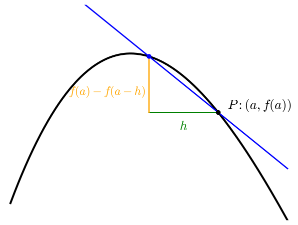
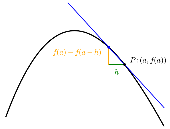
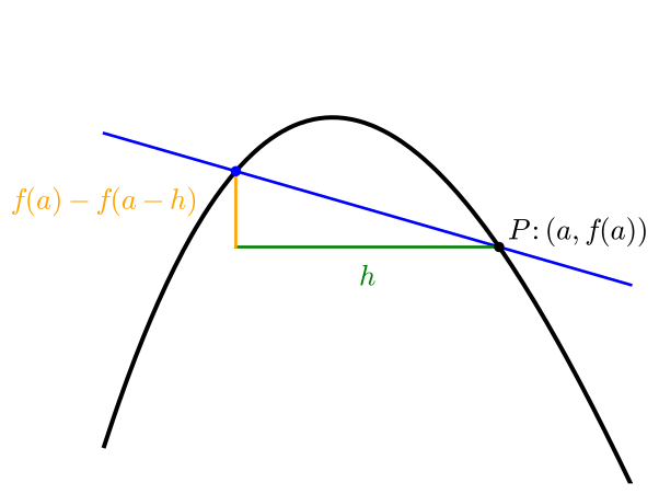
The development of the definition of the derivative is an example of the Classic Calculus Approach. In order to understand how quickly the output of a function is changing at a particular input value, we approximate with the average rate of change over an interval, which corresponds to the slope of a secant line. This approximation is step 1 of the CCA.
As the points involved in the secant line become closer to the particular input value, the approximation becomes closer to the true rate of change at the particular input value. The slope of the secant line is the difference quotient: the change in the function value divided by the change in the inputs to the function. This quantification of how the slope of the secant line changes depending on the step size of the input is step 2 of the CCA.
By looking at the limit of this difference quotient as the change in the inputs approaches zero, we can compute the true rate of change for the function.
described in detail following the image
A plot of a downward facing parabola with a blue line going between two points on the parabola. The blue line corresponds to more horizontal change than vertical change. The right point on the parabola is labeled \(P:(a,f(a))\text{.}\) The change in the vertical coordinates between these two points is represented with a vertical segment in yellow and is labeled \(f(a)-f(a-h)\text{.}\) The change in the horizontal coordinates between two points is represented by a green line segment that is labeled \(h\text{.}\)
described in detail following the image
A plot of a downward facing parabola with a blue line going between two points on the parabola. The blue line in this plot is steeper than in the previous plot and the points are closer together on the parabola. The right point on the parabola is labeled \(P:(a,f(a))\text{.}\) The change in the vertical coordinates between these two points is represented with a vertical segment in yellow and is labeled \(f(a)-f(a-h)\text{.}\) The change in the horizontal coordinates between two points is represented by a green line segment that is labeled \(h\text{.}\)
described in detail following the image
A plot of a downward facing parabola with a blue line going between two points on the parabola. The blue line in this plot is slightly steeper than in the previous plot and the two points are close together on the parabola. The right point on the parabola is labeled \(P:(a,f(a))\text{.}\) The change in the vertical coordinates between these two points is represented with a vertical segment in yellow and is labeled \(f(a)-f(a-h)\text{.}\) The change in the horizontal coordinates between two points is represented by a green line segment that is labeled \(h\text{.}\)
Algebraically, we can view this classic calculus approach as:
\begin{align*} \text{rate of change of }f \amp\approx \frac{f(a+h)-f(a)}{h} \amp \amp\text{(slope of secant line)}\\ \text{rate of change of }f \amp=\lim_{h\rightarrow 0} \frac{f(a+h)-f(a)}{h} \amp\amp \text{(slope of tangent line)} \end{align*}
Note that other derivative definitions correspond to different ways of thinking about how the two nearby points involved in the secant line approach the input of interest. The formula above approaches the point of interest from the right, but derivative formulas exist for the left difference or central difference methods. After evaluating the limit, all of these formulas calculate the same value for the derivative since there is only one instantaneous rate of change for the function at the particular input of interest.
You may not have noticed, but the limit formula for the derivative at a point is of the form of an β€œinteresting” limit because
\begin{equation*} \lim_{h\rightarrow 0} (f(a+h)-f(a)) \, \frac{1}{h} \end{equation*}
has
\begin{equation*} \lim_{h \rightarrow 0} f(a+h)-f(a)=0 \quad \text{and} \quad \frac{1}{h} \rightarrow \infty\text{ as }h \rightarrow 0\text{.} \end{equation*}
This means that we need other tools to evaluate the limit involved in derivatives.
Your first calculus course likely generalized the derivative at a point to \(f'(x)=\frac{df}{dx}\text{,}\) a function which outputs the rate of change of \(f\) for the input value \(x\text{.}\) This led to a collection of rules for efficiently calculating derivatives (e.g., power rule, sum/difference, product rule, chain rule, etc.) by thinking about the derivative \(f'(x)\) as a function related to the function \(f\text{.}\) This perspective also leads to taking derivatives of derivatives, which is often used to measure features of graphs such as concavity.
We will take moment here to note another progression of ideas that was common in single variable calculus that will be very prevalent in our work with multivariable calculus. Most calculus topics follow the progression:
  1. motivation given by the measuring a geometric feature
  2. definition developed by the Classic Calculus Approach
  3. stated definition of quantity involving limit form (which is difficult to calculate with, but explains what is being measured)
  4. introduction of algebraic rules to aid in calculation or theorem about how to efficiently calculate quantity
The concept of derivatives in single variable calculus followed this progression of ideas and ended with learning many algebraic rules about how to calculate derivatives (sum/difference rule, coefficient rule, product rule, exponent rule, etc.)

Integration.

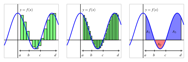
The (definite) integral of a function on an interval measures the net signed area between the graph of the function and the horizontal axis. To approximate this area, we break the interval of interest into subintervals and use rectangles whose bases are the subintervals and whose heights are determined by the function’s value at some point in the subinterval. Adding the area of these rectangles leads to an approximation of the exact area under the curve, which completes step 1 of the CCA.
By using smaller and smaller subintervals, this rectangular approximation gets closer to the exact area under the curve. We can quantify this refinement and complete step 2 of the CCA with the following equation.
\begin{align*} \text{area under the graph of }f \amp\approx \sum_{i=0}^n f(x_i^*) \Delta x_i \end{align*}
This kind of sum is referred to as a Riemann sum for the function \(f\) over the interval from \(a\) to \(b\text{.}\)
Thus, taking the limit of the sum of the areas of these rectangles as the width of all of the subintervals goes to zero gives the exact area under the curve.
\begin{align*} \text{area under the graph of }f \amp=\lim_{\Delta x_i \rightarrow 0} \sum_{i=0}^n f(x_i^*) \Delta x_i \end{align*}
described in detail following the image
A sequence of three images shows different Riemann sum converging to the definite integral. The left image shows a sinusoidal graph in blue that goes above and below the the horizontal axis. From left to right, points with inputs a, b, c, and d are labeled on a horizontal segment. The blue graph is above the horizontal axis between inputs a nd b and between c and d. The blue graph is below the horizontal axis between b and c. Eleven green rectangles extend vertically from the horizontal axis to the blue graph on the region of inputs from a to d. The center image shows a sinusoidal graph in blue that goes above and below the the horizontal axis. From left to right, points with inputs a, b, c, and d are labeled on a horizontal segment. The blue graph is above the horizontal axis between inputs a nd b and between c and d. The blue graph is below the horizontal axis between b and c. Twenty two green rectangles extend vertically from the horizontal axis to the blue graph on the region of inputs from a to d. These green rectangles better approximate the area under the blue graph, as compared to the left image. The right image shows a sinusoidal graph in blue that goes above and below the the horizontal axis. From left to right, points with inputs a, b, c, and d are labeled on a horizontal segment. The blue graph is above the horizontal axis between inputs a nd b and between c and d. The blue graph is below the horizontal axis between b and c. The area below the blue curve and above the horizontal axis for inputs from a to b is shaded in blue and labeled \(A_1\text{.}\) The area above the blue curve and below the horizontal axis for inputs from b to c is shaded in red and labeled \(A_2\text{.}\) The area below the blue curve and above the horizontal axis for inputs from c to d is shaded in blue and labeled \(A_3\text{.}\)
Your introduction to integrals likely investigated multiple rules for selecting which point you use to find the height of the rectangles in your approximation (e.g., right endpoint, left endpoint, midpoint, trapezoid etc.). However, a key idea is that the actual value of the integral does not depend on this choice.
If we use equally-sized subintervals in our approximation, then the Riemann sum argument above fits the form of our β€œinteresting” limits. Specifically,
\begin{equation*} \lim_{\Delta x \rightarrow 0} \sum_{i=0}^n f(x_i^*) \, \Delta x \end{equation*}
with
\begin{equation*} \lim_{\Delta x \rightarrow 0} \Delta x = \lim_{n \rightarrow \infty} \frac{b-a}{n} = 0 \quad \text{and} \quad \sum_{i=0}^n f(x_i^*) \rightarrow \infty\text{ as }n \rightarrow \infty \end{equation*}
Note that increasing the number of subintervals corresponds exactly with decreasing the width of these equally-sized subintervals to zero.
You may have generalized the idea of the definite integral by looking at the accumulation of a function. Recovering Position from Velocity recalls how position can be thought of as the accumulation of change in velocity. The idea of accumulation of change (not limited to velocity leading to change in position) will be important in our future study.

Recovering Position from Velocity.

Suppose that an object moves along a number line (i.e., in one dimension) with velocity given as \(v(t)\text{.}\) The object’s position is also a function of time, which we denote by \(x(t)\) so that \(x'(t) = v(t)\text{.}\) We also let \(x_0 = x(0)\text{.}\) In this framework, we can express the position at time \(t=a\) as
\begin{equation*} x(a) = x_0 + \int_{0}^a v(t)\, dt\text{.} \end{equation*}

Proof.

In many physical problems, it is easier to monitor velocity rather than position because velocity is a local measurement, while position is not a local measurement. This may seem surprising at first, so we will consider our example of piloting a car. Tracking the position of a car for all times on a trip requires a coordinate system and constant measurement of distance between the car and reference objects such as axes or coordinate planes. This requires measurement beyond the car and an external view of the car. This is why systems like GPS satellites and receivers are necessary for accurate global navigation. In contrast, note that the car does not need something outside of itself to measure its speed because the speed is a measurement of change in position relative to a small step around the current location.
Because velocity is the change in position over time, \(\text{velocity}=\frac{\Delta \text{position}}{\Delta \text{time}}\text{,}\) we can measure a change in position by multiplying velocity by the change in time (\(\Delta \text{position}=\text{velocity} \Delta \text{time}\)) if velocity is constant. Over a small time interval, velocity changes very little, or is close to constant. Therefore, we can apply this relation and use a classic calculus approach to approximate, refine, and precisely state the position as a function of time.
We know the position of the object at time \(0\) because \(x(0)=x_0\text{.}\) Thus, we want to use the velocity to measure the change in position (on the number line) between \(t=0\) and time \(t=a\text{.}\) We approximate this change in position as \(\Delta \text{position}=(\text{velocity})(\Delta \text{time})\text{.}\) To do this, we divide the interval \([0,a]\) into \(n\) equally-sized pieces of size \(\Delta t= \frac{a}{n}\text{.}\) The endpoints of these intervals are where \(t_0=0, t_1=\Delta t, \ldots, t_{n-1}=(n-1)\Delta t, t_n =a\text{.}\) The position at \(t=a\) is given by
\begin{equation*} x(a)=x_0+ \Delta x_1 + \ldots + \Delta x_n \end{equation*}
where \(\Delta x_i\) is change in position from \(t_{i-1}\) to \(t_i\text{.}\)
On each interval \([t_{i-1},t_i]\text{,}\) we evaluate the velocity at some point in the interval, denoted \(v(t_i^*)\text{,}\) and then approximate the change in position by multiplying \(v(t_i^*)\) by \(\Delta t\text{.}\) This gives us the estimate of the change in position on the interval as \(\Delta x_i \approx v(t_i^*) \Delta t \text{.}\) Our estimate of the position of our object at \(t=a\) is then
\begin{equation*} x(a)\approx x_0+\sum_{i=1}^n v(t_i^*) \Delta t \quad \quad \text{for some }t_i^*\in[t_{i-1},t_i] \text{.} \end{equation*}
This approximation is step one of the classic calculus approach.
Step 2 of the classic calculus approach requires an understanding of how this approximation works on a finer scale. A β€œfiner scale” in this case means a larger number \(n\) of subintervals. Increasing \(n\) means that \(\Delta t\) decreases. In other words, a finer scale means more terms in the sum but a smaller step size multiplier (\(\Delta t\)).
The estimate is now a Riemann sum where the function being evaluated in the Riemann sum is the velocity \(v(t)\text{.}\) Recognizing this leads to translating the Riemann sum into a definite integral as step three of the classic calculus approach. As \(n\rightarrow \infty\) or \(\Delta t \rightarrow 0\text{,}\)
\begin{equation*} x_0+\sum_{i=1}^n v(t_i^*) \Delta t \rightarrow x(a)=x_0+\int_0^{a} v(t) \, dt\text{.} \end{equation*}
In practice, this approximation is what GPS systems do at very fine level: use hyper-accurate timing and changes in relative velocities to satellites to give current position.
Accumulation will also apply to situations when working with density of a material as well. For instance, if considering a mining machine that harvests a mineral from the surface, the amount the machine harvests is the accumulation of the densities of the mineral along the path the machine followed. Mathematically this can be expressed as
\begin{align*} \text{total harvested} \amp= \sum \text{amount in each section driven} \\ \amp\approx \sum (\text{density}) (\text{length of the section}) \end{align*}
This Riemann sum becomes a definite integral of the density function in the classic calculus approach. This idea of accumulation of a function is something we will use in most chapters of the remainder of this text.