Print preview

Section 12.6 Double Integrals in Polar Coordinates

Motivating Questions

What is the area element \(dA\) in polar coordinates?
How do we convert a double integral in rectangular coordinates to a double integral in polar coordinates?

Notes to the Instructor and Dependencies.

Because we choose to cover polar coordinates in the chapter on the precalculus of multivariable functions, this section jumps right into how polar coordinates work in double integrals and provide some computational advantages. If you did not cover Section 9.9 when teaching Chapter 9, you will need to cover at least the subsection on polar coordinates before teaching this section. The preview activity in this section helps students recall important elements of points, graphs, and regions in polar coordinates before we apply the same slicing and iterated integral techniques as in Section 12.4.

This section has only two activities (plus the preview activity). For instructors who introduced polar coordinates in Chapter 9, it will be easy to cover this section in a single class meeting. Instead of having more activities in this section, we encourage instructors to reinforce that cylindrical coordinates are “polar coordinates with \(z\)” so that the section on triple integrals in cylindrical coordinates can also help students build skills in this area.

Subsection 12.6.1 Introduction

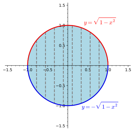
Suppose that we would like to integrate \(f(x,y) = e^{x^2 + y^2}\) over the the unit disc \(D\) centered at the origin. Using the methods we have learned thus far tin the chapter, we could evaluate this double integral using the iterated integral

\begin{equation*} \iint_D f(x,y) \, dA = \int_{x = -1}^{x = 1} \int_{y = -\sqrt{1-x^2}}^{y = \sqrt{1-x^2}} e^{x^2 + y^2} \, dy \, dx\text{.} \end{equation*}

This relies on treating \(D\) as vertically simple, as suggested in Figure 12.6.1.

described in detail following the image — Figure 12.6.1. A unit disc centered at the origin with slices showing a vertically simple description

For this particular integral, we are unable to find an antiderivative of the integrand. Changing the order of integration does not help, as the region and the integrand are symmetric in \(x\) and \(y\text{.}\) Furthermore, even if we could find an antiderivative, the inner limits of integration involve relatively complicated functions. However, the region of integration has rotational symmetry about the origin. This should make you think about polar coordinates, which we introduced in Subsection 9.9.2. In this section, we will see how we can use polar coordinates to write double integrals as iterated integrals, allowing us to both streamline the writing of the limits of integration and make evaluating the iterated integral easier.

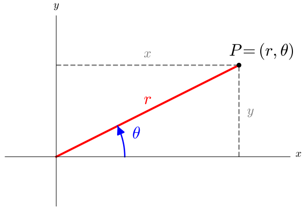
Recall that a point \(P\) in rectangular coordinates that is described by an ordered pair \((x,y)\text{,}\) where \(x\) is the displacement from \(P\) to the \(y\)-axis and \(y\) is the displacement from \(P\) to the \(x\)-axis can also be described with polar coordinates \((r,\theta)\text{,}\) where \(r\) is the distance from \(P\) to the origin and \(\theta\) is the angle formed by the line segment \(\overline{OP}\) and the positive \(x\)-axis, as shown in Figure 12.6.2.

Trigonometry and the Pythagorean Theorem allow for straightforward conversion from rectangular to polar, and vice versa. A reminder of these formulas, which were developed in Subsection 9.9.2, is included below.

Converting between rectangular and polar coordinates.

From polar to rectangular: Given polar coordinates \((r,\theta)\) of a point \(P\text{,}\) the rectangular coordinates \((x,y)\) of \(P\) satisfy

\begin{align*} x \amp = r \cos(\theta) \amp y \amp= r \sin(\theta)\text{.} \end{align*}
From rectangular to polar: Given rectangular coordinates \((x,y)\) of a point \(P\text{,}\) the polar coordinates \((r,\theta)\) of \(P\) satisfy

\begin{align*} r^2 \amp = x^2 + y^2 \amp \tan(\theta) \amp= \frac{y}{x} \text{,} \end{align*}

assuming \(x \neq 0\text{.}\)

The labels in the box above are useful when thinking about converting the coordinates of a point from one coordinate system to the other. As we think about iterated integrals, however, we will often need to take a function \(z=f(x,y)\) in which the inputs are described in rectangular coordinates and rewrite it using polar coordinates. This task simply requires using substitutions for \(x\) and \(y\) given in the first part of the conversions.

Recall that when considering polar coordinates, it is important to think about how the sign of \(r\) influences the position of a point. There are also multiple angle measurements in polar coordinates that can be used for a single point, so it will be helpful to think flexibly about ranges of \(\theta\) when describing regions in polar coordinates. Refer to Example 9.9.12 and later examples for different ways to interpret and make conversions between rectangular and polar coordinates.

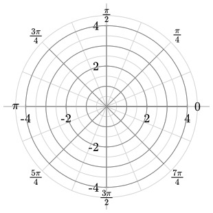
We can draw graphs of curves in polar coordinates in a similar way to how we do in rectangular coordinates. However, when plotting in polar coordinates, we use a grid that considers changes in angles and changes in distance from the origin. In particular, the angles \(\theta\) and distances \(r\) partition the plane into small wedges as shown in Figure 12.6.3.

Preview Activity 12.6.1.

This Preview Activity asks you to practice converting some equations and regions between rectangular and polar coordinates.

(a)

For each of the following polar equations, draw a plot in the plane of the curve. Write a sentence for each graph to explain why the equation is satisfied.

\(\displaystyle r=1\)
\(\displaystyle r=3\)
\(\displaystyle r=0\)
\(\displaystyle \theta =1\)
\(\displaystyle \theta = \frac{3\pi}{4}\)

(b)

Draw a plot of the region described by the following inequalities:

\begin{equation*} 1 \leq r \leq 3 \qquad\text{and}\qquad \frac{\pi}{2} \leq \theta \leq \frac{3\pi}{4} \end{equation*}

(c)

Sketch the region in the \(xy\)-plane with \(x\leq 0\text{,}\) \(y\leq 0\text{,}\) and inside the circle \(x^2+y^2=25\text{.}\) State inequalities for \(r\) and \(\theta\) that describe the region.

(d)

Sketch the region in the \(xy\)-plane that lies between the circles \(x^2+y^2=4\) and \(x^2+y^2=9\text{.}\) State inequalities for \(r\) and \(\theta\) that describe the region.

Subsection 12.6.2 Integration in Polar Coordinates

To find a way to evaluate the double integral

\begin{equation*} \iint_D e^{x^2+y^2} \, dA \end{equation*}

where \(D\) is the unit disk using polar coordinates, we will find a way to write this double integral as an iterated integral in the variables \(r\) and \(\theta\text{.}\) We will need to complete three steps to transform this double integral into polar coordinates:

Convert the area element to polar coordinates.
Describe the region of integration with inequalities that correspond to fixing one coordinate and bounding the other in a consistent way.
Convert the integrand \(f(x,y)\) to polar coordinates.

The second and third of these steps are already things we have discussed in the context of understanding polar coordinates, and we will return to them for this specific integral shortly. However, understanding how to write the area element \(dA\) in polar coordinates is a new topic. To do this, we focus on how the area element \(dA\) can be written in terms of \(dr\) and \(d\theta\) in the context of polar coordinates.

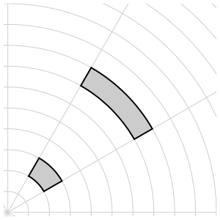
To write \(dA\) in polar coordinates, we start by remembering what \(dA\) represents. It comes from \(\Delta A\text{,}\) which is the area of the base of a rectangular prism used to approximate a volume. In rectangular coordinates, \(\Delta A = \Delta x\, \Delta y\text{,}\) which leads to \(dA = dx\, dy\text{.}\) To think in polar coordinates, we need to consider the area of a polar rectangle with \(R_0\leq r\leq R_1 \) and \(\theta_0 \leq \theta\leq \theta_1\text{.}\) Figure 12.6.4 shows two polar rectangles with the same values of \(\theta_0\) and \(\theta_1\text{.}\) However, the figure illustrates that a polar rectangle located farther from the origin has greater area than one located closer to the origin, even when \(\Delta\theta = \theta_1 - \theta_0\) and \(\Delta r = R_1 - R_0\) are the same for the two polar rectangles. This suggests that \(dA\) depends on not only \(dr\) and \(d\theta\) but also \(r\text{.}\)

Before stating and justifying the formula for \(dA\) in polar coordinates, it’s worth also thinking about what the units on \(dA\) are. They need to be units of area, so suppose that \(x\) and \(y\) are both measured in centimeters. Then \(dA = dx\, dy\) in rectangular coordinates has units square centimeters, which is an area unit. However, in polar coordinates, \(\theta\) is measured in radians. Conventionally, we treat quantities measured in radians as lacking units, so \(d\theta\, dr\) would have units of centimeters, which is a unit of length, not area.

Key Idea 12.6.5.

In polar coordinates, the area element is

\begin{equation*} dA = r \, dr\, d\theta\text{.} \end{equation*}

Proof.

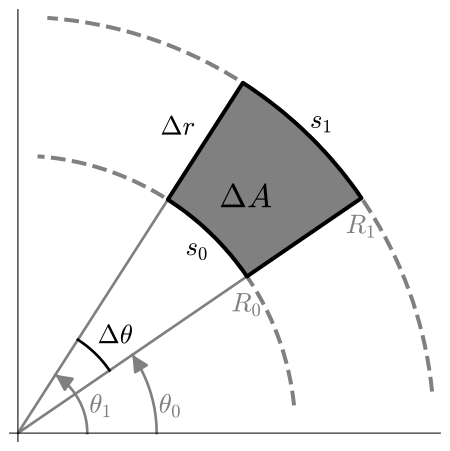
Remember that the Classic Calculus Approach to defining the double integral involved breaking each coordinate into smaller pieces which created a collection of smaller (rectangular) regions that we used to create our Riemann sum. We can do the same procedure in terms of polar coordinates, and we could have our smaller pieces be in terms of some small changes in \(r\) and \(\theta\text{,}\) such as the regions on the polar grid in Figure 12.6.3. Notice however that, as we showed in Figure 12.6.4, even though the changes in \(r\) and \(\theta\) used to define the grid are all the same, a region farther from the origin has larger area than one closer to the origin. This suggests that understanding how to measure the area of a piece described by \(R_0\leq r \leq R_1\) and \(\theta_0 \leq \theta \leq \theta_1\text{,}\) as shown in Figure 12.6.7, will be more complicated than in rectangular coordinates.

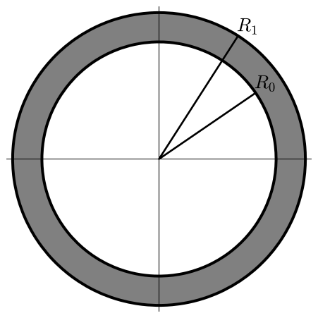
We first consider the area of the annulus between \(r=R_0\) and \(r=R_{1}\text{,}\) shown in Figure 12.6.6. The area of this region is the difference between the area of a disk of radius \(R_1\) and the area of a disk of radius \(R_0\text{:}\)

\begin{equation*} A(r=R_1)-A(r=R_0)= \pi R_1^2-\pi R_0^2=\pi\left(R_1^2-R_0^2\right) \end{equation*}

We need to measure the area of the portion of the annulus satisfying \(\theta_0 \leq \theta \leq \theta_1\text{.}\) Let \(\Delta \theta=\theta_1-\theta_0\) be the change in \(\theta\) for the small piece for which we want to find the area. Because we are using radian measures for angles, the fraction of the annulus we are considering is \(\frac{\Delta \theta}{2\pi}\text{.}\) This means that the area of this small piece is

\begin{equation*} \Delta A = \frac{\Delta \theta}{2\pi} \left(\pi\left(R_1^2-R_0^2\right)\right)\text{.} \end{equation*}

Now we can reorganize our expression for \(\Delta A\) by writing \(R_1^2-R_0^2\) as the difference of two squares. This gives

\begin{align*} \Delta A \amp= \frac{\Delta \theta}{2\pi} \left(\pi(R_1+R_0)(R_1-R_0)\right)\\ \amp= \Delta \theta \left(\frac{R_1+R_0}{2}\right) \Delta r\text{,} \end{align*}

where \(\Delta r = R_1-R_0\text{.}\) Note that as \(\Delta r \) gets smaller, \(R_1\) and \(R_0\) get closer to the same value, which means that

\begin{equation*} \Delta A \approx R_1 \Delta r \, \Delta \theta\text{.} \end{equation*}

Since we can easily convert the function \(f(x,y)\) to polar coordinates with the conversion equations to be \(f(r\cos(\theta),r\sin(\theta))\text{,}\) we can then approximate a double integral \(\iint_D f(x,y) \, dA\) with a Riemann sum of the form

\begin{align*} \iint_D f(x,y) \, dA\amp= \sum_{j=1}^n \sum_{i=1}^m f(r_i^*\cos(\theta_j^*), r_i^* \sin(\theta_j^*)) \enspace \Delta A\\ \amp= \sum_{j=1}^n \sum_{i=1}^m f(r_i^*\cos(\theta_j^*), r_i^* \sin(\theta_j^*)) \enspace r_i^*\, \Delta r \, \Delta \theta\text{.} \end{align*}

Notice that here, instead of the \(\Delta x\, \Delta y\) that we had in a Riemann sum using rectangular coordinates, our integrand is multiplied by \(r_i^*\, \Delta r\, \Delta \theta\text{.}\) This leads us to the realization that we need to use \(dA = r\, dr\, d\theta\) when writing a double integral as an iterated integral in polar coordinates.

Returning briefly to our discussion of units, notice that \(dA = r\, dr\, d\theta\) has units of square centimeters if \(x\) and \(y\) (and thus \(r\)) are measured in centimeters. This is an area unit, as desired. Before getting into describing more complicated regions in polar coordinates, we return to the example of evaluating \(\iint_D e^{x^2+y^2}\, dA\) over the unit disc \(D\text{.}\)

Example 12.6.8.

Let \(f(x,y) = e^{x^2+y^2}\) on the disk \(D = \{(x,y) : x^2 + y^2 \leq 1\}\text{.}\) Our goal in this example is to evaluate \(\displaystyle \iint_D f(x,y) \, dA\text{.}\)

In rectangular coordinates the double integral \(\iint_D f(x,y) \, dA\) can be written as the iterated integral

\begin{equation*} \iint_D f(x,y) \, dA = \int_{x=-1}^{x=1} \int_{y=-\sqrt{1-x^2}}^{y=\sqrt{1-x^2}} e^{x^2+y^2} \, dy \, dx\text{,} \end{equation*}

where the vertically simple slicing is shown in Figure 12.6.1

We cannot evaluate this iterated integral because \(e^{x^2 + y^2}\) does not have an elementary antiderivative with respect to either \(x\) or \(y\text{.}\) However, since \(r^2=x^2+y^2\) and the region \(D\) is circular, it is natural to wonder whether converting to polar coordinates will allow us to evaluate the new integral. To do so, we replace \(x\) with \(r \cos(\theta)\text{,}\) \(y\) with \(r \sin(\theta)\text{,}\) and \(dy \, dx\) with \(r \, dr \, d\theta\) to obtain

\begin{equation*} \iint_D f(x,y) \, dA = \iint_D e^{r^2} \, r \, dr \, d\theta\text{.} \end{equation*}

The disc \(D\) is described in polar coordinates by the inequalities \(0 \leq r \leq 1\) and \(0 \leq \theta \leq 2\pi\text{.}\) Therefore, it follows that

\begin{equation*} \iint_D e^{r^2} \, r \, dr \, d\theta = \int_{\theta=0}^{\theta = 2\pi} \int_{r=0}^{r=1} e^{r^2} \, r \, dr \, d\theta\text{.} \end{equation*}

We can evaluate the resulting iterated polar integral as follows:

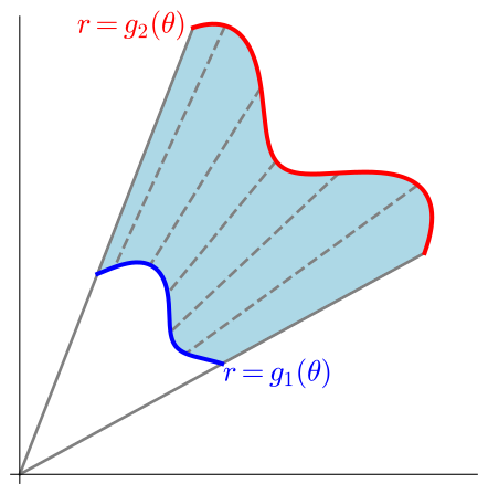
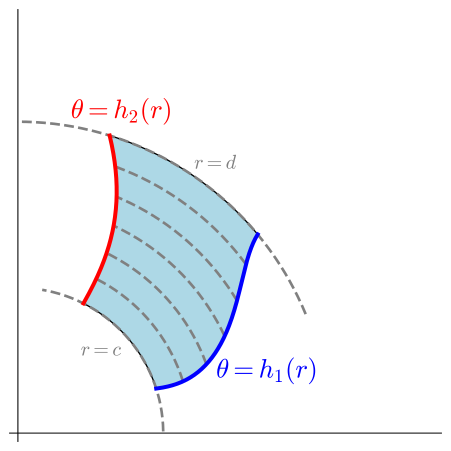
\begin{align*} \int_{\theta=0}^{\theta = 2\pi} \int_{r=0}^{r=1} e^{r^2} \, r \, dr \, d\theta \amp = \int_{\theta=0}^{2\pi} \left( \frac{1}{2}e^{r^2}\restrict{r=0}{r=1} \right) \, d\theta\\ \amp = \frac{1}{2} \int_{\theta=0}^{\theta = 2\pi} \left( e-1 \right) \, d\theta\\ \amp = \frac{1}{2}(e-1) \int_{\theta=0}^{\theta = 2\pi} \, d\theta\\ \amp = \frac{1}{2}(e-1)\left[\theta\right]\restrict{\theta=0}{\theta = 2\pi}\\ \amp = \pi(e-1)\text{.} \end{align*}

We now focus on the second conversion step: convert the region of integration described by inequalities that correspond to fixing one coordinate and bounding the other in a consistent way. Similar to how we used vertically simple and horizontally simple descriptions for rectangular regions, we want to set up inequalities by holding one of our coordinates constant and setting boundary functions for the other coordinate.

Key Idea 12.6.9.

A region is called radially simple if it can be described by a set of inequalities of the form

\begin{gather*} a \leq \theta \leq b\\ g_1(\theta) \leq r \leq g_2(\theta)\text{,} \end{gather*}

corresponding geometrically to the region in Figure 12.6.10

A region is called angularly simple if it can be described by a set of inequalities of the form

\begin{gather*} c \leq r \leq d\\ h_1(r) \leq \theta \leq h_2(r)\text{,} \end{gather*}

corresponding geometrically to the region in Figure 12.6.11

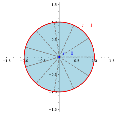
Note that the unit disc \(D\) we have considered throughout this section can be considered both radially simple and angularly simple since all of the bounds of integration are constant. Figure 12.6.12 shows how \(D\) can be considered radially simple.

Regions that are angularly simple but not radially simple do not arise with much frequency. Thus, while we have defined both types of simple regions for completeness, we will not spend time on an example of a region that is angularly simple but not radially simple.

Each of the types of regions above corresponds to exactly the necessary description to use an iterated integral. With a radially simple region, for any fixed value of \(\theta\) in the interval \([a,b]\text{,}\) a slice along this constant \(\theta\) value corresponds to a ray from the origin in the sector between the grey lines in Figure 12.6.10. Along this ray with \(\theta=k\text{,}\) the region of interest has upper and lower bounds on the \(r\)-coordinate. In fact, \(r=g_2(\theta)\) describes the upper boundary for every value of \(\theta\) in \([a,b]\text{.}\) Similarly, \(r=g_1(\theta)\) describes the lower boundary for every value of \(\theta\) in \([a,b]\text{.}\) Geometrically, this means that along every gray dashed slice where \(\theta\) is constant, the region has the same upper and lower boundary curves, shown in red and blue, respectively.

While angularly simple regions are used less frequently than radially simple regions, a parallel structure is used. Along every slice with a constant value of \(r\) in \([c,d]\text{,}\) represented by the gray, dashed curves in Figure 12.6.11, the upper bound on \(\theta\) is given by the function \(\theta=h_2(r)\) and the lower bound is given by \(\theta=h_1(r)\text{,}\) shown by the red and blue bounding curves in Figure 12.6.11.

Just as in the rectangular coordinate case, especially complicated regions may need to be split into several different regions that are radially or angularly simple.

Double integrals in polar coordinates.

The double integral \(\iint_D f(x,y) \, dA\) in rectangular coordinates can be converted to a double integral in polar coordinates as \(\iint_D f(r\cos(\theta), r\sin(\theta)) \, r \, dr \, d\theta\text{.}\)

If the region \(D\) is radially simple with \(a \leq \theta \leq b\) and \(g_1(\theta) \leq r \leq g_2(\theta)\text{,}\) then

\begin{equation*} \iint_D f(x,y) \, dA = \int_a^b \int_{g_1(\theta)}^{g_2(\theta)} f(r\cos(\theta) , r\sin(\theta)) \, r \, dr \, d\theta\text{.} \end{equation*}

If the region \(D\) is angularly simple with \(c \leq r \leq d\) and \(h_1(r) \leq \theta \leq h_2(r)\text{,}\) then

\begin{equation*} \iint_D f(x,y) \, dA = \int_c^d \int_{h_1(r)}^{h_2(r)} f(r\cos(\theta) , r\sin(\theta)) \, r \, d\theta \, dr\text{.} \end{equation*}

Note again that the order of integration corresponds to the manner in which we have sliced the region of integration. The variable being held constant along a slice is the last variable to be integrated, just as was the case with iterated integrals in rectangular coordinates.

Example 12.6.13.

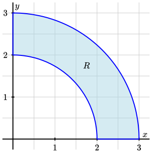
Suppose that we have a piece of metal in the shape of a quarter annulus \(R\text{,}\) as shown in Figure 12.6.14. The circular arcs bounding the region have radius \(2\) and \(3\text{,}\) and the region lies in the first quadrant. The metal is heated so that the temperature in degrees Celsius at the point \((x,y)\) is given by \(T(x,y) = \sqrt{x^2+y^2}\text{.}\) That is, the temperature is 12 times the distance between the origin and the point. In this example, we will find the average value of \(T\) over the region \(R\text{.}\)

To find the average value of \(T\) on \(R\text{,}\) we must compute

\begin{equation*} \frac{1}{\text{Area}(R)}\iint_R T\, dA\text{.} \end{equation*}

We can compute the area of \(R\) using geometry, as its area is one quarter the area of the annulus between the circles of radius \(2\) and \(3\) centered at the origin. That annulus has area \(\pi\cdot 3^2 - \pi\cdot 2^2 = 5\pi\text{,}\) so \(R\) has area \(5\pi/4\text{.}\) To compute the double integral, we will use an iterated integral. This will require finding inequalities that allow us to describe \(R\text{.}\) Notice first that \(R\) is neither horizontally simple nor vertically simple, so evaluating \(\iint_R T\, dA\) rectangular coordinates would require that we set up multiple iterated integrals. However, in polar coordinates, we see that \(R\) is both radially simple and angularly simple. That is, \(R\) is a polar rectangle, which we can describe as

\begin{equation*} 2\leq r\leq 3\qquad 0\leq \theta\leq \frac{\pi}{2}\text{.} \end{equation*}

Using this description of \(R\) in polar coordinates along with the facts that \(r^2 = x^2+y^2\) and \(dA = r\, dr, d\theta\text{,}\) we can evaluate the double integral:

\begin{align*} \iint_R T(x,y)\, dA \amp = \iint_R 12\sqrt{x^2+y^2}\, dA\\ \amp = \int_0^{\pi/2} \int_2^3 12r\cdot r\, dr\, d\theta\\ \amp = \int_0^{\pi/2} 4r^3\restrict{2}{3}\, d\theta\\ \amp = \int_0^{pi/2} 76\, d\theta = 76\theta\restrict{0}{\pi/2} = 38\pi\text{.} \end{align*}

Therefore, the average temperature of the metal plate is

\begin{equation*} \frac{1}{\frac{5\pi}{4}} 38\pi = \frac{4}{5\pi}\cdot 38\pi = \frac{152}{5} = 30.4^\circ\text{ C}\text{.} \end{equation*}

While there is no firm rule for when polar coordinates can or should be used, they are a natural alternative anytime the domain of integration may be expressed simply in polar form and/or when the integrand involves expressions such as \(\sqrt{x^2 + y^2}\text{.}\)

Activity 12.6.2.

In this activity, we will find the volume of the solid region \(V\) above the \(xy\)-plane, below the paraboloid \(z=f(x,y) = 25-x^2-y^2\text{,}\) and outside the cylinder \(x^2+y^2 = 1\text{.}\)

(a)

We will find the volume by computing a double integral \(\iint_R f(x,y)\, dA\) where \(R\) is an appropriate region in the \(xy\)-plane. Sketch the region \(R\text{.}\)

(b)

Write inequalities to describe \(R\) in polar coordinates. Write a couple of sentences explaining why it would be very difficult to describe \(R\) using rectangular coordinates.

(c)

Use an interated integral in polar coordinates to find the volume of \(V\text{.}\)

The next activity asks you to find the volume between two surfaces in three-dimensional space. To do this, you will find it useful to think of the functions involved in polar coordinates from the very beginning.

Activity 12.6.3.

Use polar coordinates to find the volume of the solid between the cone \(z=f(x,y)=\sqrt{x^2+y^2}\) and the paraboloid \(z=g(x,y)=\frac{1}{8}\left(x^2+y^2\right) + 2\text{.}\)

Perhaps the surfaces in Activity 12.6.3 brought thoughts of cylindrical coordinates to your mind. The next section will generalize the idea of a double integral to a triple integral, and after that, we will consider integration using cylindrical and spherical coordinates as well.

Summary

The area element \(dA\) in polar coordinates is determined by the area of a slice of an annulus and is given by

\begin{equation*} dA = r \, dr \, d\theta \end{equation*}
To convert the double integral \({\displaystyle\iint_D f(x,y) \, dA}\) to an iterated integral in polar coordinates, we substitute \(r \cos(\theta)\) for \(x\text{,}\) \(r \sin(\theta)\) for \(y\text{,}\) and \(r \, dr \, d\theta\) for \(dA\) to obtain the iterated integral (where the order of integration is determined by whether the region is described as radially or angularly simple)

\begin{equation*} {\iint_D f(r\cos(\theta), r\sin(\theta)) \, r \, dr \, d\theta} \end{equation*}

Exercises 12.6.3 Exercises

You can find many more problems involving the conversion of points, graphs, and region between rectangular and polar coordinates in Section 9.9. The exercises of this section will be focused on applications of these conversion to double integrals.

1.

Sketch the region of integration for the following integral.

\(\displaystyle \int_{0}^{\pi/4} \int_{0}^{6 / \cos(\theta)} f(r,\theta) \, r \, dr \, d\theta\)

The region of integration is bounded by

\(\displaystyle y = 0, y = x, \mbox{ and } y = 6\)
\(\displaystyle y = 0, y = x, \mbox{ and } x = 6\)
\(\displaystyle y = 0, y = \sqrt{36 - x^2}, \mbox{ and } x = 6\)
\(\displaystyle y = 0, x = \sqrt{36 - y^2}, \mbox{ and } y = 6\)
None of the above

2.

Convert the integral

\begin{equation*} \int_0^{\sqrt{10}}\int_{-x}^x\,dy\,dx \end{equation*}

to polar coordinates and evaluate it (use \(t\) for \(\theta\)):

With \(a =\) , \(b =\) , \(c =\) and \(d =\) ,

\(\int_0^{\sqrt{10}}\int_{-x}^x\,dy\,dx = \int_{a}^{b}\int_{c}^{d}\) \(dr\,dt\)

\(= \int_{a}^{b}\) \(\,dt\)

\(=\) \(\bigg|_{a}^{b}\)

\(=\) .

3.

For each of the following, set up the integral of an arbitrary function \(f(x,y)\) over the region in whichever of rectangular or polar coordinates is most appropriate. (Use \(t\) for \(\theta\) in your expressions.)

(a) The region

a sector of a circle of radius 4 centered at the origin, with radial endpoints (4,0) and (2,sqrt(3)2).

With \(a =\) , \(b =\) ,

\(c =\) , and \(d =\) ,

integral = \(\int_a^b \int_c^d\) \(d\) \(d\)

(b) The region

a rectangular region with diagonally opposite corners (0,4) and (2,7).

With \(a =\) , \(b =\) ,

\(c =\) , and \(d =\) ,

integral = \(\int_a^b \int_c^d\) \(d\) \(d\)

4.

By changing to polar coordinates, evaluate the integral

\begin{equation*} \iint_D (x^2 + y^2)^{7/2}\, dx dy \end{equation*}

where \(D\) is the disk \(x^2 + y^2 \le 4\text{.}\)

Answer =

5.

Using polar coordinates, evaluate the integral which gives the area which lies in the first quadrant between the circles \(x^2 + y^2 = 36\) and \(x^2 - 6x + y^2 = 0\text{.}\)

6.

(a) Graph \(r=1/(4\cos\theta)\) for \(-\pi/2\le\theta\le\pi/2\) and \(r=1\text{.}\) Then write an iterated integral in polar coordinates representing the area inside the curve \(r=1\) and to the right of \(r=1/(4\cos\theta)\text{.}\) (Use \(t\) for \(\theta\) in your work.)

With \(a =\), \(b =\),

\(c =\), and \(d =\),

area = \(\int_a^b\int_c^d\,\)\(d\) \(d\)

(b) Evaluate your integral to find the area.

area =

7.

Using polar coordinates, evaluate the integral \(\displaystyle \int \!\! \int_{R} \sin (x^2+y^2) dA\) where R is the region \(4 \leq x^2 + y^2 \leq 81\text{.}\)

8.

Use the polar coordinates to find the volume of a sphere of radius 6.

9.

Consider the solid under the graph of \(z = e^{-x^2-y^2}\) above the disk \(x^2 + y^2 \leq a^2\text{,}\) where \(a > 0\text{.}\)

(a) Set up the integral to find the volume of the solid.

Instructions: Please enter the integrand in the first answer box, typing theta for \(\theta\text{.}\) Depending on the order of integration you choose, enter dr and dtheta in either order into the second and third answer boxes with only one dr or dtheta in each box. Then, enter the limits of integration.

\(\displaystyle \int_A^B \int_C^D\)

A =

B =

C =

D =

(b) Evaluate the integral and find the volume. Your answer will be in terms of \(a\text{.}\)

Volume V =

\(\displaystyle \lim_{a \to \infty} V =\)

10.

Sketch the region whose area is given by the integral and evaluate it.

\begin{equation*} \int_{\frac{\pi}{4}}^{\frac{3\pi}{4}} \int_{3}^{8}\!\! r \,dr \,d\theta \end{equation*}

Answer:

11.

Sketch the region whose area is given by the integral and evaluate it.

\begin{equation*} \int_{0}^{\pi/2} \int_{0}^{8 \sin \theta}\!\! r \,dr \,d\theta \end{equation*}

Answer:

12.

Using polar coordinates, evaluate the integral \(\displaystyle \int \!\! \int_{R} \sin (x^2+y^2) dA\) where R is the region \(16 \leq x^2 + y^2 \leq 25\text{.}\)

13.

A cylindrical drill with radius 1 is used to bore a hole through the center of a sphere of radius 6. Find the volume of the ring shaped solid that remains.

14.

Evaluate the double integral \(\displaystyle \iint_D x^{2}y \, dA,\) where \(D\) is the top half of the disc with center the origin and radius \(4,\) by changing to polar coordinates.

Answer:

15.

Evaluate the double integral \(\displaystyle \iint_R (2 x - y) \, dA,\) where \(R\) is the region in the first quadrant enclosed by the circle \(x^2+y^2=4\) and the lines \(x=0\) and \(y=x,\) by changing to polar coordinates.

Answer:

16.

Use polar coordinates to find the volume of the solid under the cone \(z=\sqrt{x^2+y^2}\) and above the disc \(x^2+y^2 \le 16.\)

Answer:

17.

Use polar coordinates to find the volume of the solid below the paraboloid \(z=48 - 3 x^2 - 3 y^2\) and above the \(xy\)-plane.

Answer:

18.

A volcano fills the volume between the graphs \(z = 0\) and \(\displaystyle z = \frac{1}{\left( x^{2} + y^{2} \right)^{21}}\text{,}\) and outside the cylinder \(x^{2} + y^{2} = 1\text{.}\) Find the volume of this volcano.

19.

Consider the iterated integral \(I = \int_{-3}^{0} \int_{-\sqrt{9-y^2}}^{0} \frac{y}{x^2 + y^2+1} \, dx \, dy.\)

Sketch (and label) the region of integration.
Convert the given iterated integral to one in polar coordinates.
Evaluate the iterated integral in (b).
State one possible interpretation of the value you found in (c).

20.

Let \(D\) be the region that lies inside the unit circle in the plane.

Set up and evaluate an iterated integral in polar coordinates whose value is the area of \(D\text{.}\)
Determine the exact average value of \(f(x,y) = y\) over the upper half of \(D\text{.}\)
Find the exact center of mass of the lamina over the portion of \(D\) that lies in the first quadrant and has its mass density distribution given by \(\delta(x,y) = 1\text{.}\) (Before making any calculations, where do you expect the center of mass to lie? Why?)
Find the exact volume of the solid that lies under the surface \(z = 8-x^2-y^2\) and over the unit disk, \(D\text{.}\)

21.

For each of the following iterated integrals,

sketch and label the region of integration,
convert the integral to the other coordinate system (if given in polar, to rectangular; if given in rectangular, to polar), and
choose one of the two iterated integrals to evaluate exactly.

\(\displaystyle \int_{\pi}^{3\pi/2} \int_{0}^{3} r^3 \, dr \, d\theta\)
\(\displaystyle \int_{0}^{2} \int_{-\sqrt{1-(x-1)^2}}^{\sqrt{1-(x-1)^2}} \sqrt{x^2 + y^2} \, dy \, dx\)
\(\displaystyle \int_0^{\pi/2} \int_0^{\sin(\theta)} r \sqrt{1-r^2} \, dr \, d\theta.\)
\(\displaystyle \int_0^{\sqrt{2}/2} \int_y^{\sqrt{1-y^2}} \cos(x^2 + y^2) \, dx \, dy.\)

22.

Consider the circle given by \(x^2 + (y-1)^2 = 1\) as shown in Figure 12.6.15.

(a)

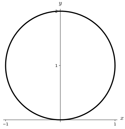
Determine a polar curve in the form \(r = f(\theta)\) that traces out the circle \(x^2 + (y-1)^2 = 1\text{.}\) To do this, you should substitute \(x = r \cos(\theta)\) and \(y = r \sin(\theta)\) into the rectangular coordinate equation and solve for \(r\text{.}\)

Hint.

After you substitute, you should expand and combine like terms. You will also want to factor your expression and disregard the \(r=0\) solution.

(b)

Find the exact average value of \(g(x,y) = \sqrt{x^2 + y^2}\) over the interior of the circle \(x^2 + (y-1)^2 = 1\text{.}\)

Hint.

Use a radially simple description of your region with your result from part a as the upper bound.

(c)

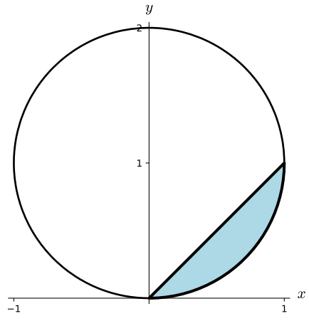
Find the volume under the surface \(h(x,y) = x\) over the region \(D\text{,}\) where \(D\) is the region bounded above by the line \(y=x\) and below by the circle. We have provided a sketch of this as the shaded region in Figure 12.6.16.

(d)

Explain why in both of the previous parts it is advantageous to use polar coordinates.

Prev Top Next

Print preview

Section 12.6 Double Integrals in Polar Coordinates

Motivating Questions

Notes to the Instructor and Dependencies.

Subsection 12.6.1 Introduction

Converting between rectangular and polar coordinates.



Preview Activity 12.6.1.

(a)

(b)

(c)

(d)

Subsection 12.6.2 Integration in Polar Coordinates

Key Idea 12.6.5.

Proof.

Example 12.6.8.

Key Idea 12.6.9.

Double integrals in polar coordinates.

Example 12.6.13.



Activity 12.6.2.

(a)

(b)

(c)



Activity 12.6.3.

Summary

Exercises 12.6.3 Exercises

1.

2.

3.

4.

5.

6.

7.

8.

9.

10.

11.

12.

13.

14.

15.

16.

17.

18.

19.

20.

21.

22.

(a)

(b)

(c)

(d)