Active Calculus - Multivariable

Section 12.1 Double Riemann Sums and Double Integrals over Rectangles

Subsection 12.1.1 Introduction

In single-variable calculus, recall that we used the classic calculus approach to define the definite integral as the area under a graph. Specifically, we approximated the area under the graph of a positive function \(f\) on an interval \([a,b]\) by adding areas of rectangles whose heights are determined by the curve. We then broke the interval \([a,b]\) into smaller subintervals, constructing rectangles on each of these smaller intervals to approximate the region under the curve on that subinterval, then summing the areas of these rectangles to approximate the area under the curve. We defined the definite integral of \(f\) using the limit of this Riemann sum as the size of all of the subintervals goes to zero.
In the Preview Activity, we will review a few ideas from integrals in single variable calculus. The rest of this section will then be used to extend the ideas of integration and its interpretations to functions of two variables over a rectangular region.

Preview Activity 12.1.1.
(a)
A plot of \(f\) for inputs in the interval \([0,2]\) is shown in Figure 12.1.1. Break the interval \([0,2]\) into four equally sized subintervals and draw the rectangles that would be used to construct a Riemann sum to approximate the area under \(f\) on the interval \([0,2]\text{.}\) You can use whichever point you want on each subinterval to evaluate the height the of the rectangles.
described in detail following the image
A continuous function on \([0,2]\)
Figure 12.1.1. A continuous function on \([0,2]\)
(b)
Estimate the heights of the rectangles used in your Riemann sum above to estimate \(\displaystyle{\int_0^2 f(x)\enspace dx}\text{.}\) Write a couple of sentences about why you think your estimate for the definite integral of \(f\) is either an overestimate, an underestimate, or close to the true value.
(c)
Recall that the definite integral is defined as
\begin{equation*} \int_a^b f(x) \enspace dx = \lim_{\Delta x_i \to 0} \sum_{i=1}^n f(x_i^*)\Delta x_i\text{.} \end{equation*}
Explain why it doesn’t matter what method (left endpoint, right endpoint, midpoint, etc.) you use for selecting which point is evaluated on each of the subintervals in the definition of the definite integral.
(d)
For each of the functions plotted below, determine if the definite integral over the region shown will be positive, negative, or zero and write a sentence to justify your answer.
described in detail following the image
ADD ALT TEXT TO THIS IMAGE
described in detail following the image
ADD ALT TEXT TO THIS IMAGE
described in detail following the image
ADD ALT TEXT TO THIS IMAGE
In this section, we will use the classic calculus approach to define and understand the definite integral for a function of two variables over a rectangular region of input values. Just as in single-variable calculus, we will develop some algebraic methods to help efficiently evaluate these integrals. Later in this chapter we will will generalize to regions that are not rectangular and work with functions of three or more variables.

Subsection 12.1.2 Double Riemann Sums over Rectangles

The motivating interpretation of a definite integral for a function of one variable was the area under a curve over a particular interval of input values. We will use the same motivating interpretation for the definite integral of function of two variables. The definite integral of a nonnegative function of two variables will measure the volume of the region beneath the graph of \(f\) over a region of input points. We can show this geometrically as the volume of the solid below the surface given by \(z=f(x,y)\) as shown in Figure 12.1.2. The surface given by \(z=f(x,y)\) is shown in blue and the region of inputs above which we want to find the volume is shown in red in the \(xy\)-plane. The double integral of \(f\) over the red region should measure the volume of the solid shaded in gray.
Figure 12.1.2. A plot of the volume under as surface \(z=f(x,y)\) over a region \(R\text{,}\) in red
The region shaded red in Figure 12.1.2 is irregular in the coordinates (\(x\) and \(y\)). We will explore this kind of problem in Section 12.3 once we have some intuition and tools from examining rectangular regions of integration. To discuss how to approach rectangular regions, we apply the classic calculus approach to the region shown in Figure 12.1.3. In particular, for this rectangular region of input points, we want to
  1. estimate the volume between the blue surface plot and the \(xy\)-plane,
  2. quantify how this estimate for the volume of the solid under the graph of \(f(x,y)\) changes when we use a smaller scale, and
  3. use a limit to find the exact value of the volume under the surface.
To estimate the volume under the graph, we will use rectangular prisms because their volume is easy to compute:
\begin{equation*} \text{Volume of rectangular prism}= (\text{length})(\text{width})(\text{height}) \end{equation*}
Figure 12.1.3. A plot of the volume under a surface over a rectangular region
In the next activity, we will go through these steps for a particular function and rectangular region of integration as well as introduce some of the notation used in our development of double integrals.

Activity 12.1.2.
In this activity, we will go through the first two steps of the classic calculus approach to compute the definite integral of \(f(x,y) = 100 - x^2-y^2\) on the rectangular domain \(R = [0,8] \times [2,6]\text{.}\) Remember that we are trying to measure the volume below the graph of \(f\) over the region \(R\text{,}\) so we will start with estimating this volume.
(a)
To understand the numerical calculations involved in the classic calculus approach for a double integral, it is most important to understand the region of integration. Thus, we will not look a graph of \(z=f(x,y)\text{.}\) Instead, we will stay focused in the \(xy\)-plane. On the axes below, outline the rectangular region \(R\) that corresponds to the region of integration.
described in detail following the image
ADD ALT TEXT TO THIS IMAGE
(b)
Because all of the regions and subregions we are considering in this section are rectangles, we can break up the \(x\) and \(y\) coordinates into pieces separately. For this activity, break the interval of \(x\)-coordinates into four equally-sized subintervals and break the interval of \(y\)-coordinates into three equally-sized subintervals.
What is the length of each subinterval in the \(x\)-direction? How about in the \(y\)-direction?
(c)
Let \(S_i\) be the \(i\)-th subinterval for \(x\text{.}\) We want to state the endpoints of each of the \(S_i\text{.}\) The first subinterval, \(S_1\text{,}\) will go from \(x_0\) to \(x_1\text{,}\) the second subinterval, \(S_2\text{,}\) will go from \(x_1\) to \(x_2\text{,}\) the third subinterval, \(S_3\text{,}\) will go from \(x_2\) to \(x_3\text{,}\) and the fourth subinterval, \(S_4\text{,}\) will go from \(x_3\) to \(x_4\text{.}\)
Give the values for \(x_0\text{,}\) \(x_1\text{,}\) \(x_2\text{,}\) \(x_3\text{,}\) and \(x_4\) and add these as tick marks on the \(x\)-axis of the graph in part a to make sure your subintervals are equally sized.
(d)
Let \(T_i\) be the \(i\)-th subinterval for \(y\text{.}\) Give the values for \(y_0\text{,}\) \(y_1\text{,}\) \(y_2\text{,}\) and \(y_3\) and add these as tick marks on the \(y\)-axis of the graph in part a to make sure your subintervals are equally sized.
(e)
We will use the subintervals in the \(x\)- and \(y\)-coordinates to specify smaller rectangles into which \(R\) is divided to compute an approximation. Let \(R_{i j}\) be the rectangle corresponding to \(S_i \times T_j\text{.}\)
  1. How many smaller rectangles are there in this partition?
  2. Outline each of the smaller rectangles on the graph in part a and label each rectangle as either \(R_{1 1}, R_{1 2} , ...\text{.}\)
  3. Since each smaller rectangle \(R_{i j}\) has the same area, let \(\Delta A\) denote the area of each of these smaller rectangles. What is \(\Delta A\text{?}\)
(f)
To find the volume of the rectangular prisms over each \(R_{i j}\text{,}\) we must pick a point in each subrectangle at which to evaluate \(f\text{,}\) which will be the height of the rectangular prism. For this activity, we will use the upper-right corner of each subrectangle as the designated point.
State the point at the upper right of each smaller rectangle and evaluate \(f\) at each of these points.
(g)
Write a sentence about why the volume of each rectangular prism used for this approximation is
\begin{equation*} f(x_i,y_j) \Delta A\text{.} \end{equation*}
Write a couple sentences about how you would find an approximation of the volume under the surface \(z=f(x,y)\) over the region \(R\text{.}\) (Do not do calculation, but rather explain what calculation is being done.)
(h)
We chose the upper-right point of each subrectangle \(R_{i j}\) to find the height of each rectangular prism used in the approximation. Write a sentence or two about whether you think the upper right point provides an overestimate, an underestimate, or approximately the average value for \(f\) on each \(R_{i j}\text{.}\) Explain how this suggests that your estimate for the volume under the surface \(z=f(x,y)\) over the region \(R\) is either an overestimate, an underestimate, or approximately the correct value.

Subsection 12.1.3 Double Riemann Sums and Double Integrals

Every part of the previous activity can be generalized to work on any bounded rectangular region using any number of subintervals in either the \(x\) or \(y\) directions. This leads us to state these steps in general below and note that using more subintervals corresponds to estimating on a smaller scale, which is step 2 of the classic calculus approach.

Definition 12.1.4.

Let \(f\) be a continuous function on a rectangle \(R = \{(x,y) : a \leq x \leq b, c \leq y \leq d\}\text{.}\) A double Riemann sum for \(f\) over \(R\) is created as follows.
  1. Partition the interval \([a, b]\) into \(m\) subintervals of equal length \(\Delta x = \frac{b-a}{m}\text{.}\) Let \(x_0\text{,}\) \(x_1\text{,}\) \(\ldots\text{,}\) \(x_m\) be the endpoints of these subintervals, where \(a = x_0\lt x_1\lt x_2 \lt \cdots \lt x_m = b\text{.}\)
  2. Partition the interval \([c, d]\) into \(n\) subintervals of equal length \(\Delta y = \frac{d-c}{n}\text{.}\) Let \(y_0\text{,}\) \(y_1\text{,}\) \(\ldots\text{,}\) \(y_n\) be the endpoints of these subintervals, where \(c = y_0\lt y_1\lt y_2 \lt \cdots \lt y_n = d\text{.}\)
  3. These two partitions create a partition of the rectangle \(R\) into \(mn\) subrectangles \(R_{ij}\) with opposite vertices \((x_{i-1},y_{j-1})\) and \((x_i, y_j)\) for \(i\) between \(1\) and \(m\) and \(j\) between \(1\) and \(n\text{.}\) These rectangles all have equal area \(\Delta A = \Delta x \cdot \Delta y\text{.}\)
  4. Choose a point \((x_{ij}^*, y_{ij}^*)\) in each rectangle \(R_{ij}\text{.}\) A double Riemann sum for \(f\) over \(R\) is given by
    \begin{equation*} \sum_{j=1}^n \sum_{i=1}^m \left(f(x_{ij}^*, y_{ij}^*) \cdot \Delta A\right)\text{.} \end{equation*}
If \(f(x,y) \geq 0\) on the rectangle \(R\text{,}\) we may ask to find the volume of the solid bounded above by \(f\) over \(R\text{,}\) as illustrated in Figure 12.1.5.
Figure 12.1.5. The solid below a surface \(z=f(x,y)\) over a rectangular region
This volume is approximated by a Riemann sum, which sums the volumes of the rectangular prisms shown in Figure 12.1.6. In a double Riemann sum, both \(m\) and \(n\) go to infinity. This means that the number of subrectangles increases without bound, as illustrated in Figure 12.1.6. As this happens, the sum of the volumes of the rectangular boxes approaches the true volume of the solid bounded above by \(z=f(x,y)\) over the region \(R\text{.}\) Use the sliders at the top of Figure 12.1.6 to change the number of subintervals used in the Riemann sum and verify geometrically how the estimated volume will approach true volume under \(f\) as \(n\) and \(m\) become arbitrarily large.
Figure 12.1.6. The estimated volume under a surface \(z=f(x,y)\) when using \(m\) by \(n\) subrectangles
The third step in the classic calculus approach is to take the limit, and when this limit exists, its value is the double integral we have been seeking:

Definition 12.1.7.

Let \(R\) be a rectangular region in the \(xy\)-plane and \(f\) a continuous function over \(R\text{.}\) With terms defined as in a double Riemann sum, the double integral of \(f\) over \(R\) is
\begin{equation*} \iint_R f(x,y) \, dA = \lim_{m,n \to \infty} \sum_{j=1}^n \sum_{i=1}^m f(x_{ij}^*, y_{ij}^*) \cdot \Delta A. \end{equation*}

Aside

For the solid shown in Figure 12.1.6, the exact volume is \(231/64 = 3.609375\text{.}\) Go back and see how close the estimate of the volume provided by the double Riemann sum is to the exact value for the largest values of \(n\) and \(m\) the sliders will allow.
We conclude this subsection by noting a couple of useful ideas in the development of double integrals that can simplify some aspects. Many times we will use equally-sized subintervals or pieces of our region of integration but that is not strictly necessary. The most general form of a double integral requires only that as we take the limit, the area of every smaller piece goes to zero. In Activity 12.1.2, we used the upper right point of each smaller rectangle to evaluate \(f\) but in Definition 12.1.7 there is not a particular point in each smaller rectangle used. Remember that as the area of all the smaller rectangles is going to zero, there will be smaller and smaller differences between the output of \(f\) on the points in the smaller rectangle.

Subsection 12.1.4 Interpretation of Double Riemann Sums and Double integrals

We conclude this section with three important interpretations of the double integral that will appear repeatedly throughout the rest of this book. We summarize these three interpretations in the Key Idea below and then discuss each in greater depth.

Signed Volume.

Suppose that \(f(x,y)\) assumes both positive and negatives values on the rectangle \(R\text{,}\) as shown in Figure 12.1.9. When constructing a Riemann sum, for each \(i\) and \(j\text{,}\) the product \(f(x_{ij}^*, y_{ij}^*) \enspace \Delta A\) can be interpreted as a “signed” volume of a box with base area \(\Delta A\) and “signed” height \(f(x_{ij}^*, y_{ij}^*)\text{.}\) Since \(f\) can have negative values, this “height” could be negative. The sum
\begin{equation*} \sum_{j=1}^n \sum_{i=1}^m f(x_{ij}^*, y_{ij}^*) \enspace \Delta A \end{equation*}
can then be interpreted as a sum of “signed” volumes of boxes, with a negative sign attached to those boxes whose heights are below the \(xy\)-plane.
Figure 12.1.9. A plot of the surface \(z=f(x,y)\) over the rectangular region \(R\)
We can then realize the double integral \(\displaystyle\iint_R f(x,y) \, dA\) as a difference in volumes: \(\iint_R f(x,y) \, dA\) tells us the volume of the solids the graph of \(f\) bounds above the \(xy\)-plane over the rectangle \(R\) minus the volume of the solids the graph of \(f\) bounds below the \(xy\)-plane under the rectangle \(R\text{.}\) This is shown in Figure 12.1.10.
Figure 12.1.10. A plot of the signed volume with the volume above the \(xy\)-plane shown in blue and the volume below the \(xy\)-plane shown in red
The double integral of \(f\) over the rectangle \(R\) will be positive because there is more volume above the \(xy\)-plane (shown in blue) thanvolume below the \(xy\)-plane, which is counted as negative and shown in red.

Activity 12.1.3.
Let \(f(x,y) = \sqrt{4-y^2}\) on the rectangular region \(R = [1,7] \times [-2,2]\text{.}\) Suppose that we partition \([1,7]\) into 3 subintervals of equal length and \([-2,2]\) into 2 subintervals of equal length. A table of values of \(f\) at some points in \(R\) is given in Table 12.1.11, and a graph of \(f\) with the indicated partitions is shown in Figure 12.1.12.
Table 12.1.11. Table of values of \(f(x,y) = \sqrt{4-y^2}\text{.}\)
\(x \downarrow \backslash \, y \rightarrow\) \(-2\) \(-1\) \(0\) \(1\) \(2\)
\(1\) \(0\) \(\sqrt{3}\) \(2\) \(\sqrt{3}\) \(0\)
\(2\) \(0\) \(\sqrt{3}\) \(2\) \(\sqrt{3}\) \(0\)
\(3\) \(0\) \(\sqrt{3}\) \(2\) \(\sqrt{3}\) \(0\)
\(4\) \(0\) \(\sqrt{3}\) \(2\) \(\sqrt{3}\) \(0\)
\(5\) \(0\) \(\sqrt{3}\) \(2\) \(\sqrt{3}\) \(0\)
\(6\) \(0\) \(\sqrt{3}\) \(2\) \(\sqrt{3}\) \(0\)
\(7\) \(0\) \(\sqrt{3}\) \(2\) \(\sqrt{3}\) \(0\)
Figure 12.1.12.
(a)
Sketch the region \(R\) in the plane partitioned as described above.
(b)
Calculate the double Riemann sum using the given partition of \(R\) and the values of \(f\) in the upper right corner of each subrectangle.
(c)
Use geometry to calculate the exact value of \(\displaystyle\iint_R f(x,y) \, dA\) and compare it to your approximation. Write a sentence to describe one way to obtain a better approximation using the given data.

Density Functions.

If the function being integrated is a density function, then the double integral measures how much of the substance being measured is in the region of integration. You can see a single-variable calculus explanation of this in Recovering Position from Velocity, and we will explore this more in the multivariable setting in Section 12.4 and later applications.
As a brief example here, if \(f\) measures the density of some material on a rectangular plot of land, then the double integral of this function will measure the total amount of that material on the plot of land. The function \(f(x,y)\) will have units of mass (of the material) per unit area and the Riemann sum
\begin{equation*} \sum_{j=1}^n \sum_{i=1}^m \left(f(x_{ij}^*, y_{ij}^*)\cdot \Delta A\right) \end{equation*}
will have units of mass. This idea is used for the laminar masses given in Section 12.4 and applies to other settings such as electric charge, which has the possibility of negative values for both the density and total amount.

Average Value.

The average of \(mn\) values \(f(x_{ij}^*, y_{ij}^*)\) of a function of two variables can be expressed as a double sum:
\begin{equation*} \text{Avg} _{mn} = \frac{1}{mn} \sum_{j=1}^n \sum_{i=1}^m f(x_{ij}^*, y_{ij}^*) \end{equation*}
If we take the limit as \(m\) and \(n\) go to infinity, we obtain what we can define as the average value of \(f\) over the region \(R\)
Although the double sum expression for \(\text{Avg}_{mn}\) appears to be missing an essential component to recognize it as a double Riemann sum that corresponds to a double integral, we can do some algebra to adjust for that. First, note that
\begin{equation*} \Delta x = \frac{b-a}{m} \quad \quad \text{ and } \quad \quad \Delta y = \frac{d-c}{n}\text{.} \end{equation*}
Thus,
\begin{equation*} \frac{1}{mn} = \frac{\Delta x \cdot \Delta y}{(b-a)(d-c)} = \frac{\Delta A}{\text{area of }R},\text{.} \end{equation*}
Then, the average value of the function \(f\) over \(R\text{,}\) which we denote by \(f_{\operatorname{AVG}(R)}\text{,}\) is given by
\begin{align*} f_{\operatorname{AVG}(R)} \amp = \lim_{m,n \to \infty} \frac{1}{mn} \sum_{j=1}^n \sum_{i=1}^m f(x_{ij}^*, y_{ij}^*)\\ \amp = \lim_{m,n \to \infty} \frac{1}{A(R)} \sum_{j=1}^n \sum_{i=1}^m f(x_{ij}^*, y_{ij}^*) \cdot \Delta A\\ \amp = \frac{1}{\text{area of }R} \iint_R f(x,y) \, dA. \end{align*}
Therefore, the double integral of \(f\) over \(R\) divided by the area of \(R\) is the average value of the function \(f\) on \(R\text{.}\)
As an additional note, if \(f(x, y) \geq 0\) on \(R\text{,}\) then we can interpret this average value of \(f\) on \(R\) as the height of the box with base \(R\) that has the same volume as the volume of the surface \(z=f(x,y)\) over \(R\text{.}\)
Activity 12.1.4.
Let \(f(x,y) = x+2y\) and let \(R = [0,2] \times [1,3]\text{.}\)
(a)
Draw a picture of \(R\text{.}\) Partition \([0,2]\) into 2 subintervals of equal length and the interval \([1,3]\) into two subintervals of equal length. Draw these partitions on your picture of \(R\) and label the resulting subrectangles using the labeling scheme we established in the definition of a double Riemann sum.
(b)
For each \(i\) and \(j\text{,}\) let \((x_{ij}^*, y_{ij}^*)\) be the midpoint of the rectangle \(R_{ij}\text{.}\) Identify the coordinates of each \((x_{ij}^*, y_{ij}^*)\text{.}\) Draw these points on your picture of \(R\text{.}\)
(c)
Calculate the Riemann sum
\begin{equation*} \sum_{j=1}^n \sum_{i=1}^m f(x_{ij}^*, y_{ij}^*) \cdot \Delta A \end{equation*}
using the partitions we have described. If we let \((x_{ij}^*, y_{ij}^*)\) be the midpoint of the rectangle \(R_{ij}\) for each \(i\) and \(j\text{,}\) then the resulting Riemann sum is called a midpoint sum.
(d)
Explain the meaning of the sum you just calculated in terms of each of the interpretations in Key Idea 12.1.8

Subsection 12.1.5 Properties of Double Integrals

We conclude this section with a list of properties of double integrals. Since similar properties are satisfied by single-variable integrals and the arguments for double integrals are essentially the same, we omit their justification.

Properties of Double Integrals.

Let \(f\) and \(g\) be continuous functions on a rectangle \(R = \{(x,y) : a \leq x \leq b, c \leq y \leq d\}\text{,}\) and let \(k\) be a constant. Then
  1. \(\displaystyle\iint_R \left(f(x,y) + g(x,y)\right) \, dA = \iint_R f(x,y) \, dA + \iint_R g(x,y) \, dA\text{.}\)
  2. \(\displaystyle\iint_R kf(x,y) \, dA = k \iint_R f(x,y) \, dA\text{.}\)
  3. If \(f(x,y) \geq g(x,y)\) on \(R\text{,}\) then \(\displaystyle\iint_R f(x,y) \, dA \geq \iint_R g(x,y) \, dA\text{.}\)

Exercises 12.1.6 Exercises

1.

Suppose \(f(x,y) = 25-x^{2}-y^{2}\) and \(R\) is the rectangle with vertices (0,0), (6,0), (6,4), (0,4). In each part, estimate \(\displaystyle \iint\limits_R f(x,y) \, dA\) using Riemann sums. For underestimates or overestimates, consistently use either the lower left-hand corner or the upper right-hand corner of each rectangle in a subdivision, as appropriate.
(a) Without subdividing \(R\text{,}\)
Underestimate =
Overestimate =
(b) By partitioning \(R\) into four equal-sized rectangles.
Underestimate =
Overestimate =

2.

Consider the solid that lies above the square (in the \(xy\)-plane) \(R = [0, 1] \times [0, 1]\text{,}\) and below the elliptic paraboloid \(z = 100 - x^2+ 6 xy - 2 y^2\text{.}\)
Estimate the volume by dividing \(R\) into 9 equal squares and choosing the sample points to lie in the midpoints of each square.

3.

Let \(R\) be the rectangle with vertices \((0,0)\text{,}\) \((2,0)\text{,}\) \((2,2)\text{,}\) and \((0,2)\) and let \(f(x,y) = \sqrt{0.25xy}\text{.}\)
(a) Find reasonable upper and lower bounds for \(\int_{R}f\,dA\) without subdividing \(R\text{.}\)
upper bound =
lower bound =
(b) Estimate \(\int_{R}f\,dA\) three ways: by partitioning \(R\) into four subrectangles and evaluating \(f\) at its maximum and minimum values on each subrectangle, and then by considering the average of these (over and under) estimates.
overestimate: \(\int_{R}f\,dA \approx\)
underestimate: \(\int_{R}f\,dA \approx\)
average: \(\int_{R}f\,dA \approx\)

4.

Using Riemann sums with four subdivisions in each direction, find upper and lower bounds for the volume under the graph of \(f(x,y) = 4+xy\) above the rectangle \(R\) with \(0\le x\le 1,\quad 0\le y \le 5\text{.}\)
upper bound =
lower bound =

5.

Consider the solid that lies above the square (in the xy-plane) \(R = [0, 2] \times [0, 2]\text{,}\)
and below the elliptic paraboloid \(z = 36 - x^{2} - 2y^2\text{.}\)
(A) Estimate the volume by dividing R into 4 equal squares and choosing the sample points to lie in the lower left hand corners.
(B) Estimate the volume by dividing R into 4 equal squares and choosing the sample points to lie in the upper right hand corners..
(C) What is the average of the two answers from (A) and (B)?

6.

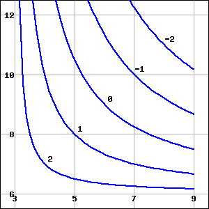
The figure below shows contours of \(g(x,y)\) on the region \(R\text{,}\) with \(5 \le x\le 11\) and \(2 \le y\le 8\text{.}\)
Using \(\Delta x = \Delta y =2\text{,}\) find an overestimate and an underestimate for \(\int_R g(x,y)\, dA\text{.}\)
Overestimate =
Underestimate =

7.

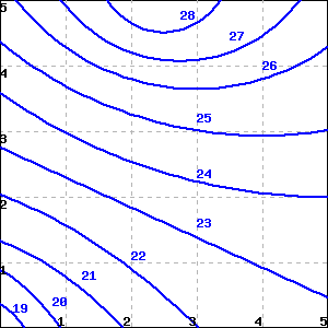
The figure below shows the distribution of temperature, in degrees C, in a 5 meter by 5 meter heated room.
Using Riemann sums, estimate the average temperature in the room.
average temperature =

8.

Values of \(f(x,y)\) are given in the table below. Let \(R\) be the rectangle \(1 \leq x \leq 1.6, 2 \leq y \leq 3.2\text{.}\) Find a Riemann sum which is a reasonable estimate for \(\int_R f(x,y) \, da\) with \(\Delta x = 0.2\) and \(\Delta y = 0.4\text{.}\) Note that the values given in the table correspond to midpoints.
\begin{equation*} \begin{array}{|c || c|c|c|} \hline y \backslash x \amp 1.1 \amp 1.3 \amp 1.5 \\ \hline \hline 2.2 \amp 4 \amp 0 \amp -5 \\ \hline 2.6 \amp -3 \amp 0 \amp 8 \\ \hline 3.0 \amp 6 \amp 6 \amp -4 \\ \hline \end{array} \end{equation*}
\(\int_R f(x,y) \, da \approx\)

9.

Values of \(f(x,y)\) are shown in the table below.
\(x = 3\) \(x = 3.2\) \(x = 3.4\)
\(y = 5\) 7 8 11
\(y = 5.4\) 6 7 8
\(y = 5.8\) 5 6 17
Let \(R\) be the rectangle \(3 \leq x \leq 3.4\text{,}\) \(5 \leq y \leq 5.8\text{.}\) Find the values of Riemann sums which are reasonable over- and under-estimates for \(\int_R f(x,y) \,dA\) with \(\Delta x=0.2\) and \(\Delta y=0.4\text{.}\)
over-estimate:
under-estimate:

10.

The temperature at any point on a metal plate in the \(xy\) plane is given by \(T(x,y) = 100-4x^2 - y^2\text{,}\) where \(x\) and \(y\) are measured in inches and \(T\) in degrees Celsius. Consider the portion of the plate that lies on the rectangular region \(R = [1,5] \times [3,6]\text{.}\)
  1. Estimate the value of \(\iint_R T(x,y) \, dA\) by using a double Riemann sum with two subintervals in each direction and choosing \((x_i^*, y_j^*)\) to be the point that lies in the upper right corner of each subrectangle.
  2. Determine the area of the rectangle \(R\text{.}\)
  3. Estimate the average temperature, \(T_{\operatorname{AVG}(R)}\text{,}\) over the region \(R\text{.}\)
  4. Do you think your estimate in (c) is an over- or under-estimate of the true temperature? Why?

11.

Let \(f\) be a function of independent variables \(x\) and \(y\) that is increasing in both the positive \(x\) and \(y\) directions on a rectangular domain \(R\text{.}\) For each of the following situations, determine if the double Riemann sum of \(f\) over \(R\) is an overestimate or underestimate of the double integral \(\iint_R f(x,y) \, dA\text{,}\) or if it impossible to determine definitively. Provide justification for your responses.
  1. The double Riemann sum of \(f\) over \(R\) where \(f\) is evaluated at the lower left point of each subrectangle.
  2. The double Riemann sum of \(f\) over \(R\) where \(f\) is evaluated at the upper right point of each subrectangle.
  3. The double Riemann sum of \(f\) over \(R\) where \(f\) is evaluated at the midpoint of each subrectangle.
  4. The double Riemann sum of \(f\) over \(R\) where \(f\) is evaluated at the lower right point of each subrectangle.

12.

The wind chill, as frequently reported, is a measure of how cold it feels outside when the wind is blowing. In Table 12.1.13, the wind chill \(w=w(v,T)\text{,}\) measured in degrees Fahrenheit, is a function of the wind speed \(v\text{,}\) measured in miles per hour, and the ambient air temperature \(T\text{,}\) also measured in degrees Fahrenheit. Approximate the average wind chill on the rectangle \([5,35] \times [-20,20]\) using 3 subintervals in the \(v\) direction, 4 subintervals in the \(T\) direction, and the point in the lower left corner in each subrectangle.
Table 12.1.13. Wind chill as a function of wind speed and temperature.
\(v \backslash T\) \(-20\) \(-15\) \(-10\) \(-5\) \(0\) \(5\) \(10\) \(15\) \(20\)
\(5\) \(-34\) \(-28\) \(-22\) \(-16\) \(-11\) \(-5\) \(1\) \(7\) \(13\)
\(10\) \(-41\) \(-35\) \(-28\) \(-22\) \(-16\) \(-10\) \(-4\) \(3\) \(9\)
\(15\) \(-45\) \(-39\) \(-32\) \(-26\) \(-19\) \(-13\) \(-7\) \(0\) \(6\)
\(20\) \(-48\) \(-42\) \(-35\) \(-29\) \(-22\) \(-15\) \(-9\) \(-2\) \(4\)
\(25\) \(-51\) \(-44\) \(-37\) \(-31\) \(-24\) \(-17\) \(-11\) \(-4\) \(3\)
\(30\) \(-53\) \(-46\) \(-39\) \(-33\) \(-26\) \(-19\) \(-12\) \(-5\) \(1\)
\(35\) \(-55\) \(-48\) \(-41\) \(-34\) \(-27\) \(-21\) \(-14\) \(-7\) \(0\)

13.

Consider the box with a sloped top that is given by the following description: the base is the rectangle \(R = [0,4] \times [0,3]\text{,}\) while the top is given by the plane \(z = p(x,y) = 20 - 2x - 3y\text{.}\)
  1. Estimate the value of \(\iint_R p(x,y) \, dA\) by using a double Riemann sum with four subintervals in the \(x\) direction and three subintervals in the \(y\) direction, and choosing \((x_i^*, y_j^*)\) to be the point that is the midpoint of each subrectangle.
  2. What important quantity does your double Riemann sum in (a) estimate?
  3. Suppose it can be determined that \(\iint_R p(x,y) \, dA = 138\text{.}\) What is the exact average value of \(p\) over \(R\text{?}\)
  4. If you wanted to build a rectangular box (with the same base) that has the same volume as the box with the sloped top described here, how tall would the rectangular box have to be?